
ULTRAVIOLET EFFECTS on PHYTOPLANKTON
Miles Mathis' Charge Field :: Miles Mathis Charge Field :: The Charge Field Effects on Humans/Animals

ULTRAVIOLET EFFECTS on PHYTOPLANKTON
![]() by Chromium6 Sun May 24, 2020 5:59 pm
by Chromium6 Sun May 24, 2020 5:59 pm
‐----
ULTRAVIOLET EFFECTS on PHYTOPLANKTON
Donat-P. Häder
Neue Str. 9, 91096 Möhrendorf, Germany
donat@dphaeder.de

Aquatic ecosystems cover about 70% of the surface of our globe. They produce an amount of biomass that is equal to all the terrestrial ecosystems (e.g., forests and grassland, agricultural areas and tundras and taigas) taken together. The oceans represent the largest share in the aquatic ecosystems, and all freshwater surfaces combined (lakes, rivers) account for only 0.5%. While macroalgae (kelp) are the major biomass producers in coastal areas, phytoplankton are the predominant players in the open sea.
Left to right: Asterinella, Biddulphia, Ceratium fusca, Coscinodiscus
While usually being microscopically small and often unicellular, these organisms grow at a fast pace, and often divide once a day. Sometimes they form dense algal blooms, which stain the water, Figure 1.
Figure 1. Phytoplankton bloom.
Phytoplankton, as the primary producers in the aquatic habitats, form the basis of the intricate aquatic food web, Figure 2. They serve the primary consumers (zooplankton such as larval fish and shrimp) as food, which in turn are consumed by the secondary consumers (crustaceans, molluscs, fish, birds and mammals including man). Thus, they ultimately provide a significant share of the world’s animal protein for human consumption, and in some parts of the world more than 50 % of the animal protein comes from the sea. The third major component in aquatic ecosystems, in addition to primary producers and consumers are the decomposers, mainly bacteria, which break down living or dead biomass into inorganic building blocks ready for reentry into the cycle.
Figure 2. Marine Food Web. Phytoplankton are the primary producers. They are consumed by zooplankton which are, in turn, consumed by progressively larger aquatic organisms. The cycle completes as nutrients from deomposing organisms circulate to supply nutritiion to phytoplankton.
Phytoplankton organisms are a major sink for atmospheric carbon dioxide (CO2) and play a key role with respect to global warming, Figure 3.
Figure 3. Global carbon fluxes and reservoir. The figure shows production (up arrows) and consumption (down arrows) of carbon by (from left to right) aquatic organisms, terrestrial organisms, industrial activity and forest fires. The biological pump refers to carbon settling to the ocean bottom in the form of decaying small particulate organic matter.
They absorb an estimated 100,000,000,000 tons, or 100 Gt (1 Gt = 1 gigaton = 109 tons) of carbon from the total reservoir of 735 Gt in the atmosphere (in the form of carbon dioxide). Most of this is recycled back into the atmosphere when the organisms decay or, after being eaten, the consumers decay. But part of the organic carbon sediments to the deep sea floor where it is stored for hundreds of thousands of years, Figure 4.
Figure 4. CO2 transport in the sea. Two carbon cycles are depicted that operate on vastly different time scales. Photosynthesis and respiration cycles carbon into and out of the ocean on a time scale measure in days. Dissolved organic carbon (DOC) and particulate organic carbon (POC) accomplish the same cycling, but measured on a time scale of centuries.
This sedimenting particulate organic carbon (POC), called “oceanic snow”, can be collected and analyzed by traps installed at defined depths (e.g. 1000 m) in the water column. This downward transport of carbon out of the system is called the “biological pump” and partially counterbalances the manmade input of carbon dioxide into the atmosphere by fossil fuel combustion and tropical deforestation. The phytoplankton is not equally distributed in the world’s oceans. Highest concentrations are found in the subpolar regions and in the upwelling areas of the continental shelves. This distribution can best be seen from satellite images which show the chlorophyll concentration in the water in false color images, Figure 5.
Figure 5. This false color image shows that the greatest phytoplankton densities are near the poles and along continental shelves. The scale in the upper reight corner indicates that blue is low density; green and yellow are higher densities.
Being photosynthetic organisms, phytoplankton are forced to move to, and to stay in, the top layer of the water column illuminated by solar radiation, the “photic zone”. The photic zone is not defined by its vertical extension in meters but rather by the amount of available solar radiation. The lower limit of the photic zone is the depth were the penetrating light decreases to 0.1 % of the surface irradiation.
The availability of light depends on several factors. The spectrum of light changes with depth as solar radiation penetrates to depth. This is due to the absorption and scattering by the water itself as well as dissolved and particulate organic and inorganic matter in the water column. In coastal areas and freshwater ecosystems dissolved organic carbon (DOC) plays a major role in attenuating the light penetration and influencing the water color. DOC is a mixture of organic compounds resulting from the breakdown of lignins, chlorophylls and other organic material washed into the water by terrestrial runoff. DOC strongly absorbs in the UV range of the spectrum. These organic compounds are consumed by the bacterioplankton; however, bacteria find it difficult to consume long-chained DOC. Solar UV breaks down these long molecules, and the bacteria can consume the fragments faster. This increases the transparency of the water and the penetration of solar UV to greater depths. One feedback loop is that solar UV damages the bacteria, decreasing their numbers.
Photomovement of Phytoplankton
Several phytoplankton organisms use active mechanisms to move to and stay in the photic zone: some have flagella or cilia and actively move in the water column in search for optimal conditions for growth and reproduction. Others use buoyancy for vertical migrations producing oil droplets or gas vacuoles. Some of these movements follow a circadian rhythm with organisms moving down at night and toward the surface before and during daytime. Several members of the dinoflagellates have been found to swim 35 m up and down in the water column during their daily movements.
Phytoplankton organisms use environmental signals to control their movements. Some bacteria follow the magnetic field lines of the Earth (magnetotaxis). Flagellates are known to detect thermal and chemical gradients of oxygen and carbon dioxide. The most important clues are light and gravity. In darkness actively motile phytoplankton organisms move upward along the gravitational field of the Earth. This behaviour is called negative gravitaxis (away from the center of gravity). This orientation mechanism is truly remarkable. These unicellular organisms perform the task of orienting in space, a task for which humans use a complicated apparatus in their inner ear and a good amount of brain power. The upward behaviour is supported by positive phototaxis (movement toward the light) in the presence of low irradiance light. Many motile phytoplankton organisms possess molecular photoreceptors and an internal signal transduction mechanism to control their motor apparatus and to orient with respect to the light direction.
In contrast to the positive phototaxis just described, many phytoplankton cannot tolerate the bright, unfiltered solar radiation at the ocean's surface and are impaired especially by the high-energy, short-wavelength radiation in the UV range of the spectrum. As a consequence, they use negative phototaxis (movement away from a light source) or reversal of their gravitaxis to move away from the water surface with its excessive detrimental radiation. These antagonistic responses, which control upward and downward orientation, result in an accumulation of the organisms in a zone of intermediate and optimal light conditions, Figure 6.
Figure 6. Phytoplankton near the ocean's surface can be harmed by solar UV. Negative Phototaxis in this intense environment causes migration to lower depths. If the phytoplankton are too deep insufficient illumination causes a positive phototactic response, so the organisms move upward to an optimal position. These vertical migrations can be overruled by the action of wind and waves.
Of course, these vertical migrations can be overruled by the action of wind and waves in the top layer of the oceans, called the “mixing layer.” The mixing layer extends from the surface downward to the level of colder, unmixed water. The boundary between these layers is called a thermocline. Even then the organisms bias their distribution in the top layer of the ocean by active or passive oriented movements.
More at link: http://photobiology.info/Hader.html
Chromium6- Posts : 729
Join date : 2019-11-29
Re: ULTRAVIOLET EFFECTS on PHYTOPLANKTON
![]() by Chromium6 Tue May 26, 2020 2:43 am
by Chromium6 Tue May 26, 2020 2:43 am
NASA has warned that Earth’s North and South magnetic poles are about to flip, causing worldwide blackouts and lethal levels of radiation to sweep over the planet.
Historically, the poles have flipped every 200,000 to 300,000 years. It has been 780,000 years since they last flipped – meaning that a shift is massively overdue. According to scientists at NASA, the planet is showing signs that a shift is imminent.
Yahoo News reports: Our planet’s magnetic field protects us from lethal levels of radiation from phenomena like solar rays. The dangerous particles never hit us directly, because upon entering the Earth’s atmosphere the magnetic field deflects them and forces them to move around, according to NASA.
So the prospect of that field weakening, which it does when it’s getting ready to flip, is worrisome: It would leave us without sufficient protection.
The Earth’s North magnetic pole has been wandering at 10-year intervals from 1970 to 2020, as seen in this animation from the National Centers for Environmental Information. NOAA National Centers for Environmental Information.
The Earth’s magnetic field extends out from electrical currents created by the metals in its core, generating invisible lines that touch back down at the planet’s opposing magnetic poles. Cosmic radiation expert Daniel Baker, director of the Laboratory for Atmospheric and Space Physics at the University of Colorado, Boulder, believes that the next pole reversal could likely render some areas of the planet unlivable, according to Undark.
That devastation could arrive through multiple avenues. The combination of powerful space particles, like unfiltered solar rays, cosmic rays and ultraviolet B rays (the stuff your sunscreen bottle warns you about), would smash through our battered ozone layer and lead us the way of the dinosaurs.
Our infrastructure wouldn’t fare much better. Since satellite grids are linked, once radiation eats through, more will follow, causing a cascading mass blackout, among other disasters, according to Undark.
Because we haven’t reached that point yet, scientists are using imagery from satellites to track the magnetic field’s movements. Since 2014, Swarm—a trio of satellites from the European Space Agency—has allowed researchers to study changes building at the Earth’s core, where the magnetic field is generated.
Their observations reveal that both the molten iron and nickel are draining out of the Earth’s core. That kind of restless activity could indicate that the field is preparing to flip, according to Undark. Protective measures could include building more radiation-fortified satellites, plus shoring up ones that are already operational, according to the International Business Times.
Not all of the Earth’s polarity reversal attempts are successful; the poles last put out a botched effort around 40,000 years ago, according to Futurism. And scientists have yet to establish a cause-and-effect relationship between pole reversals and mass extinctions.
https://newspunch.com/nasa-earths-poles-flip/
Chromium6- Posts : 729
Join date : 2019-11-29
Re: ULTRAVIOLET EFFECTS on PHYTOPLANKTON
![]() by Chromium6 Tue May 26, 2020 2:45 am
by Chromium6 Tue May 26, 2020 2:45 am
Extremely powerful cosmic rays are raining down on us. No one knows where they come from.
But with large-scale experiments, scientists around the world are determined to find out.
By Brian Resnick@B_resnickbrian@vox.com Updated Jul 25, 2019, 7:17am EDT
Graphics: Javier Zarracina/Vox
The Highlight by Vox logo
You may think the greatest, most perplexing mysteries of the universe exist way out there, at the edge of a black hole, or inside an exploding star.
No, great mysteries of the universe surround us, all the time. They even permeate us, sailing straight through our bodies. One such mystery is cosmic rays, made of tiny bits of atoms. These rays, which are passing through us at this very moment, are not harmful to us or any other life on the surface of Earth.
But some carry so much energy that physicists are baffled by what object in the universe could have created them. Many are much too powerful to have originated from our sun. Many are much too powerful to have originated from an exploding star. Because cosmic rays don’t often travel in a straight line, we don’t even know where in the night sky they are coming from.
The answer to the mystery of cosmic rays could involve objects and physical phenomena in the universe that no one has ever seen or recorded before. And physicists have several enormous experiments around the world underway now devoted to cracking the case.
Though we don’t know where they come from, or how they get here, we can see what happens when these cosmic rays hit our planet’s atmosphere at nearly the speed of light.
Cosmic rays are messengers from the broader universe; a reminder we’re a part of it, and a reminder that there’s still a great deal of mystery out there. Let’s take a close look at these astonishing particles, raining on Earth from afar.
Smashing into our atmosphere
When the particles in cosmic rays collide with the atoms in at the top of the atmosphere, they burst, tearing apart atoms in a violent collision. The particles from that explosion then keep bursting apart other bits of matter, in a snowballing chain reaction. Some of this atomic shrapnel even hits the ground.
Javier Zarracina/Vox
A depiction of cosmic rays hitting the earth.
Javier Zarracina/Vox; NASA
It’s possible to see this in action by building what’s called a cloud chamber out of a glass jar, felt, dry ice, and isopropyl alcohol (i.e. rubbing alcohol). You soak the felt in the alcohol, and the dry ice (which is super-cold solid carbon dioxide) cools down the alcohol vapor, which is streaming down from the felt. That creates a cloud of alcohol vapor.
In this chamber, you can see the cosmic rays, particularly those from a particle called a muon. Muons are like electrons, but a bit heavier. Every square centimeter of Earth at sea level, including the space at the top of your head, gets hit by one muon every minute.
Like electrons, muons carry a negative charge. When the muons zip through the alcohol cloud, they ionize (charge) the air they pass through. The charge in the air attracts the alcohol vapor, and it condenses into droplets. And those droplets then trace the path the cosmic rays made through the chamber.
When you see the paths these muons make, think about this: These subatomic particles rocket down to Earth at 98 percent the speed of light.
They move so fast, they experience the time dilation predicted by Einstein’s theory of special relativity. They’re supposed to decay — i.e. break apart into smaller components, electrons, and neutrinos — in just 2.2 microseconds, which would mean they’d barely get 2,000 feet down from the top of the atmosphere before dying. But because they’re moving so fast, relative to us, they age 22 times more slowly. (A similar thing happened to Matthew McConaughey’s character in the movie Interstellar, as he sped up his relative speed nearing a black hole.)
If Einstein’s theory weren’t true, we wouldn’t see any muons in the cloud chamber. Luckily, they are harmless, moving so fast that they don’t have the time to land an impactful punch in your body. Scientists can do some cool things with muons, like use them to photograph the inside of the Great Pyramid in Egypt.
Recall that these rays were potentially propelled by forces from beyond our solar system, by forces no physicist understands. That’s plainly awesome
https://www.vox.com/the-highlight/2019/7/16/17690740/cosmic-rays-universe-theory-science
Chromium6- Posts : 729
Join date : 2019-11-29
Re: ULTRAVIOLET EFFECTS on PHYTOPLANKTON
![]() by LongtimeAirman Tue May 26, 2020 10:14 pm
by LongtimeAirman Tue May 26, 2020 10:14 pm
Thanks for the selection Cr6. They do seem to go well together. You had me hooked with the Phytoplankton, a life form that change its ocean depth in order to reduce the amount of solar energy it receives sounds like a fine biological charge engine to me.
Cr6 wrote. Pole flip news...a bit alarmist
Airman. Un huh, the Pole flip news is what prompted me to reply. Regions becoming unlivable, possibly an extinction event? Alarmist indeed. I wasn’t aware of some of the nonsense it is handing out.Yahoo News reports: Our planet’s magnetic field protects us from lethal levels of radiation from phenomena like solar rays. The dangerous particles never hit us directly, because upon entering the Earth’s atmosphere the magnetic field deflects them and forces them to move around, according to NASA.
So the prospect of that field weakening, which it does when it’s getting ready to flip, is worrisome: It would leave us without sufficient protection.
https://milesmathis.forumotion.com/t598-what-does-miles-intend-by-the-classification-photon-vs-anti-photon#6197
Airman. I should have thanked you for your extremely pertinent question/comment a week and a half ago. Answering it warmed me up for this comment.Cr6 wrote. has Miles mentioned any connection between +/- photon flows and magnetic reversals? If flows are disrupted then poles reverse?
The flipping of the magnetic poles does not expose us surface dwellers to increased high energy solar emissions. As Miles has explained, the unequal ratio of charge/anti-charge, two to one here on earth as the solar system passes through this part of the galaxy is the source of earth’s strong magnetic field. The availability and ratio of charge and anti-charge received by the earth can vary. If that ratio were to change to one to one, as might occur during a magnetic pole flip, the earth’s emissions and atmosphere resistance to incoming solar energy doesn’t shut off. Recall Miles describing the fact that Venus has a very low magnetic field, even though Venus’ emissions are stronger than the earth’s.
Of course there are many other false ideas contained in this story, such as magnetic field lines which extend outside the earth, from pole to pole. I’ll stop there.
The third story, Extremely powerful cosmic rays are raining down on us is good for general knowledge. Someone standing at sea level will receive a muon a minute due to cosmic rays. There are many high energy particle detectors, with job openings for those who would wish to similar work world wide. I like the simple instructions on building one's own cloud chamber high energy particle detector. I basically have one comment, they seem to imply that some cosmic rays have almost limitless energy and so they are a “mystery”. According to the charge field, We know e=mc^2; if we know the size and speed of a particle, we know exactly how much energy it can contain and why.
.
LongtimeAirman- Admin
- Posts : 2030
Join date : 2014-08-10
Re: ULTRAVIOLET EFFECTS on PHYTOPLANKTON
![]() by Chromium6 Wed May 27, 2020 2:03 am
by Chromium6 Wed May 27, 2020 2:03 am
Actually wikipidia has some detail on this. I take wikipedia with a grain of salt since they tend to overlook certain factors in their commentary. During this "flip" eras..does the earth explode in hydrocarbon formation in the seas? If more UV light hits the earth then sensitive plankton just grows and PAHs are trapped:
https://amesteam.arc.nasa.gov/Publications/docs/Gudipati_Allamandola_2004.pdf
---------------
Photochemical degradation of hydroxy PAHs in ice: Implications for the polar areas
Author links
Gea1
JunLib1
Guangshui
NaaChang-ErChenc
2 ChengHuoaPengZhanga
ZiweiYaoa
https://doi.org/10.1016/j.chemosphere.2016.04.087
Highlights
• It is first reported on photochemical behaviour of 4 hydroxylated PAHs in ice.
• Photolysis kinetics varied substantially due to different structures and properties.
• Photoinduced hydroxylation formed multiple hydroxylated intermediates.
• Photodegradation is prominent in determining the OH-PAH fate in polar sunlit snow/ice.
Abstract
Hydroxyl polycyclic aromatic hydrocarbons (OH-PAHs) are derived from hydroxylated PAHs as contaminants of emerging concern. They are ubiquitous in the aqueous and atmospheric environments and may exist in the polar snow and ice, which urges new insights into their environmental transformation, especially in ice. In present study the simulated-solar (λ > 290 nm) photodegradation kinetics, products and pathways of four OH-PAHs (9-Hydroxyfluorene, 2-Hydroxyfluorene, 1-Hydroxypyrene and 9-Hydroxyphenanthrene) in ice were investigated, and the corresponding implications for the polar areas were explored. It was found that the kinetics followed the pseudo-first-order kinetics with the photolysis quantum yields (Φs) ranging from 7.48 × 10⁻³ (1-Hydroxypyrene) to 4.16 × 10⁻² (2-Hydroxyfluorene). These 4 OH-PAHs were proposed to undergo photoinduced hydroxylation, resulting in multiple hydroxylated intermediates, particularly for 9-Hydroxyfluorene. Extrapolation of the lab data to the real environment is expected to provide a reasonable estimate of OH-PAH photolytic half-lives (t1/2,E) in mid-summer of the polar areas. The estimated t1/2,E values ranged from 0.08 h for 1-OHPyr in the Arctic to 54.27 h for 9-OHFl in the Antarctic. In consideration of the lower temperature and less microorganisms in polar areas, the photodegradation can be a key factor in determining the fate of OH-PAHs in sunlit surface snow/ice. To the best of our knowledge, this is the first report on the photodegradation of OH-PAHs in polar areas.
https://www.sciencedirect.com/science/article/pii/S004565351630577X
-----------

Geomagnetic polarity since the middle Jurassic. Dark areas denote periods where the polarity matches today's polarity, while light areas denote periods where that polarity is reversed. The Cretaceous Normal superchron is visible as the broad, uninterrupted black band near the middle of the image.
https://en.wikipedia.org/wiki/Geomagnetic_reversal
..............
Geomagnetic polarity time scale
Further information: Magnetostratigraphy
Through analysis of seafloor magnetic anomalies and dating of reversal sequences on land, paleomagnetists have been developing a Geomagnetic Polarity Time Scale (GPTS). The current time scale contains 184 polarity intervals in the last 83 million years (and therefore 183 reversals).[10][11]
Changing frequency over time
The rate of reversals in the Earth's magnetic field has varied widely over time. 72 million years ago (Ma), the field reversed 5 times in a million years. In a 4-million-year period centered on 54 Ma, there were 10 reversals; at around 42 Ma, 17 reversals took place in the span of 3 million years. In a period of 3 million years centering on 24 Ma, 13 reversals occurred. No fewer than 51 reversals occurred in a 12-million-year period, centering on 15 million years ago. Two reversals occurred during a span of 50,000 years. These eras of frequent reversals have been counterbalanced by a few "superchrons" – long periods when no reversals took place.[12]
Superchrons
A superchron is a polarity interval lasting at least 10 million years. There are two well-established superchrons, the Cretaceous Normal and the Kiaman. A third candidate, the Moyero, is more controversial. The Jurassic Quiet Zone in ocean magnetic anomalies was once thought to represent a superchron, but is now attributed to other causes.
The Cretaceous Normal (also called the Cretaceous Superchron or C34) lasted for almost 40 million years, from about 120 to 83 million years ago, including stages of the Cretaceous period from the Aptian through the Santonian. The frequency of magnetic reversals steadily decreased prior to the period, reaching its low point (no reversals) during the period. Between the Cretaceous Normal and the present, the frequency has generally increased slowly.[13]
The Kiaman Reverse Superchron lasted from approximately the late Carboniferous to the late Permian, or for more than 50 million years, from around 312 to 262 million years ago.[13] The magnetic field had reversed polarity. The name "Kiaman" derives from the Australian village of Kiama, where some of the first geological evidence of the superchron was found in 1925.[14]
The Ordovician is suspected to have hosted another superchron, called the Moyero Reverse Superchron, lasting more than 20 million years (485 to 463 million years ago). Thus far, this possible superchron has only been found in the Moyero river section north of the polar circle in Siberia.[15] Moreover, the best data from elsewhere in the world do not show evidence for this superchron.[16]
Certain regions of ocean floor, older than 160 Ma, have low-amplitude magnetic anomalies that are hard to interpret. They are found off the east coast of North America, the northwest coast of Africa, and the western Pacific. They were once thought to represent a superchron called the Jurassic Quiet Zone, but magnetic anomalies are found on land during this period. The geomagnetic field is known to have low intensity between about 130 Ma and 170 Ma, and these sections of ocean floor are especially deep, causing the geomagnetic signal to be attenuated between the seabed and the surface.[16]
Duration
Most estimates for the duration of a polarity transition are between 1,000 and 10,000 years,[13] but some estimates are as quick as a human lifetime.[23] Studies of 16.7-million-year-old lava flows on Steens Mountain, Oregon, indicate that the Earth's magnetic field is capable of shifting at a rate of up to 6 degrees per day.[24] This was initially met with skepticism from paleomagnetists. Even if changes occur that quickly in the core, the mantle, which is a semiconductor, is thought to remove variations with periods less than a few months. A variety of possible rock magnetic mechanisms were proposed that would lead to a false signal.[25] However, paleomagnetic studies of other sections from the same region (the Oregon Plateau flood basalts) give consistent results.[26][27] It appears that the reversed-to-normal polarity transition that marks the end of Chron C5Cr (16.7 million years ago) contains a series of reversals and excursions.[28] In addition, geologists Scott Bogue of Occidental College and Jonathan Glen of the US Geological Survey, sampling lava flows in Battle Mountain, Nevada, found evidence for a brief, several-year-long interval during a reversal when the field direction changed by over 50 degrees. The reversal was dated to approximately 15 million years ago.[29][30] In August 2018, researchers reported a reversal lasting only 200 years.[31] But a 2019 paper estimated that the most recent reversal, 780,000 years ago, lasted 22,000 years.[32][33]
Hypothesized triggers
Some scientists, such as Richard A. Muller, think that geomagnetic reversals are not spontaneous processes but rather are triggered by external events that directly disrupt the flow in the Earth's core. Proposals include impact events[40][41] or internal events such as the arrival of continental slabs carried down into the mantle by the action of plate tectonics at subduction zones or the initiation of new mantle plumes from the core-mantle boundary.[42] Supporters of this hypothesis hold that any of these events could lead to a large scale disruption of the dynamo, effectively turning off the geomagnetic field. Because the magnetic field is stable in either the present North-South orientation or a reversed orientation, they propose that when the field recovers from such a disruption it spontaneously chooses one state or the other, such that half the recoveries become reversals. However, the proposed mechanism does not appear to work in a quantitative model, and the evidence from stratigraphy for a correlation between reversals and impact events is weak. There is no evidence for a reversal connected with the impact event that caused the Cretaceous–Paleogene extinction event.[43]
...............
In the new study, the researchers relied on flow sequences of lava that erupted close to or during the last reversal, to measure its duration. Using this method, they estimated that the reversal lasted 22,000 years — much longer than the previous estimates of 1,000 to 10,000 years.
"We found that the last reversal was more complex, and initiated within the Earth's outer core earlier, than previously thought," lead study author Bradley Singer, a professor of geoscience at the University of Wisconsin-Madison, told Space.com.
While conducting studies on a volcano in Chile in 1993, Singer stumbled upon one of the lava-flow sequences that recorded part of the reversal process. While trying to date the lava, Singer noticed odd, transitional magnetic-field directions in the lava-flow sequences.
"Such records are indeed extremely rare, and I am one of very few people who date them," Singer said.
Since then, he's made it his career-long goal to better explain the timing of magnetic-field reversals.
The reversals take place when iron molecules in Earth's spinning outer core start going in the opposite direction as other iron molecules around them. As their numbers grow, these molecules offset the magnetic field in Earth's core. (If this were to happen today, it would render compasses useless as the needle would swing from pointing towards the north pole to pointing to the south.)
Click here for more Space.com videos...
During this process, Earth's magnetic field, which protects the planet from hot sun particles and solar radiation, becomes weaker.
"This kind of duration would mean the shielding of the Earth from solar radiation would be very complex and, on average, less effective over a longer time period," John Tarduno, a professor of geophysics at the University of Rochester who was not involved in the study, told Space.com. "The actual effects of that are still debatable, and they're not as tragic or as extreme as someone might suggest, but there still can be important effects."
Some of these effects, Singer suggested, could include genetic mutations or additional stress on certain animal or plant species, or possible extinctions, due to increased exposure to harmful ultraviolet light from the sun. An increase in particles from the sun entering Earth's atmosphere could also cause disruption to satellites and other communication systems, like radio and GPS, he added.
Recent reports of the magnetic field jolting from the Canadian Arctic toward Siberia have sparked debate over whether the next magnetic-field reversal is imminent and what kind of impact that would have on life on Earth.
However, Singer dismissed these claims. "There is little evidence that this current decrease in field strength, or the rapid shift in position of the north pole, reflect behavior that portends a polarity reversal is imminent during the next 2,000 years," he said.
Using the data gathered from lava flows, geologists can learn a lot more about magnetic-field reversals. "Even though volcanic records are not complete records, they're still the best kind of records we have of recording a given time and place," Tarduno said. "Higher accuracy in the age dating, and being able to get more detailed records [of the reversals]...will give the community a lot to think about," he added.
https://www.space.com/lava-flows-earth-magnetic-field-reversal.html
----------
Chromium6- Posts : 729
Join date : 2019-11-29
Re: ULTRAVIOLET EFFECTS on PHYTOPLANKTON
![]() by Chromium6 Wed May 27, 2020 2:27 am
by Chromium6 Wed May 27, 2020 2:27 am
By Passant Rabie August 07, 2019
Volcanic records revealed the complexity of the magnetic-field reversal.
Earth's north and south magnetic poles flip-flop over long timescales. New research into volcanic rocks may explain how it happens.
(Image:
The last reversal of Earth's magnetic poles happened long before humans could record it, but research on the flow of ancient lava has helped scientists estimate the duration of this strange phenomenon.
A team of researchers used volcanic records to study Earth's last magnetic-field reversal, which occurred about 780,000 years ago. They found that this flip may have taken much longer than researchers previously thought, the scientists reported in a new study.
Earth's magnetic field has flipped dozens of times in the past 2.5 million years, with north becoming south and vice versa. Scientists know the last reversal took place during the Stone Age, but they have little information about the duration of this phenomenon and when the next "flip" might occur.
https://www.space.com/41604-magnetic-field-rapid-reversal.html
-----------
Earth's Magnetic Field Can Reverse Poles Ridiculously Quickly, Study Suggests
By Brandon Specktor August 23, 2018
https://www.space.com/41604-magnetic-field-rapid-reversal.html
------------
Death by UV? Did an increase in UV radiation kill off the soft-bodied creatures of the Ediacaran—pictured—paving the way for the Cambrian explosion?
Chase Studio/Science Source
Hyperactive magnetic field may have led to one of Earth’s major extinctions
By Ian RandallFeb. 16, 2016 , 10:45 AM
Rapid reversals of Earth’s magnetic field 550 million years ago destroyed a large part of the ozone layer and let in a flood of ultraviolet radiation, devastating the unusual creatures of the so-called Ediacaran Period and triggering an evolutionary flight from light that led to the Cambrian explosion of animal groups. That’s the conclusion of a new study, which proposes a connection between hyperactive field reversals and this crucial moment in the evolution of life.
The Kotlinian Crisis, as it is known, saw widespread extinction and put an end to the Ediacaran Period. During this time, large (up to meter-sized) soft-bodied organisms, often shaped like discs or fronds, had lived on or in shallow horizontal burrows beneath thick mats of bacteria which, unlike today, coated the sea floor. The slimy mats acted as a barrier between the water above and the sediments below, preventing oxygen from reaching under the sea floor and making it largely uninhabitable.
The Ediacaran gave way to the Cambrian explosion, 542 million years ago: the rapid emergence of new species with complex body plans, hard parts for defense, and sophisticated eyes. Burrowing also became more common and varied, which broke down the once-widespread bacterial mats, allowing oxygen into the sea floor to form a newly hospitable space for living.
Scientists have long argued over what caused the Cambrian explosion in the first place. Potential explanations have included rising levels of atmospheric oxygen because of photosynthesis, allowing for the development of more complex animals; the rise in carnivorous species and new predatory tactics, such as the flat and segmented, armor-crushing creatures known as anomalocaridids; and the breakup of the supercontinent Rodinia, which may have created new ecological niches and isolated populations as the continents drifted apart.
In their new study, however, geologist Joseph Meert of the University of Florida in Gainesville and his colleagues propose a different hypothesis: that these evolutionary changes might have been connected to rapid reversals in the direction of Earth’s magnetic field. During a reversal, magnetic north and south trade places—an event which, in geologically recent times, occurs about once every million years.
Yet in the Ediacaran, such reversals were a lot more common, the team proposes. Certain minerals in rocks can preserve a record of the direction of Earth’s magnetic field when the rock formed. While studying these magnetic records in 550-million-year-old, Ediacaran-aged sedimentary rocks in the Ural Mountains in western Russia, the team discovered evidence to suggest the reversal rate then was 20 times faster than it is today. “Earth’s magnetic field underwent a period of hyperactive reversals,” Meert says.
Previous research has suggested that Earth’s protective magnetic field would be weaker across such periods of frequent reversal, compromising its ability to shield life from harmful solar radiation and cosmic rays. On top of this, the duration of each individual reversal episode—thought to take an average of 7000–10,000 years—would likely see the field temporarily weakened even more before growing back in the opposite direction.
This weakened shielding would have allowed more energetic particles into the upper atmosphere, which would have begun to break down the ozone layer that protects Earth from harmful UV radiation, Meert says. Twenty to 40% of ozone coverage might have been lost—in turn, doubling the amount of UV radiation that reached Earth’s surface, the team reports in a paper in press in Gondwana Research. “Organisms with the ability to escape UV radiation would be favored in such an environment.”
This flight from dangerous levels of UV light, therefore, might explain many of the evolutionary changes that occurred during the Late Ediacaran and Early Cambrian, Meert says. Creatures with complex eyes to sense the light and the ability to seek shelter from the radiation—for example, by migrating into deeper waters during the daytime—would have been more successful. The growth of hard coatings and shells would afford additional UV protection, as would the capacity to burrow deeper into the sea floor.
In turn, these changes may have opened up new environments. The development of shells, for example, helps creatures colonize intertidal areas, protected not only from UV rays but also stronger waves and the risk of drying out. Similarly, the breakdown of the bacterial mats by early burrowing would have opened up the upper sea floor further for life.
https://www.sciencemag.org/news/2016/02/hyperactive-magnetic-field-may-have-led-one-earth-s-major-extinctions
Chromium6- Posts : 729
Join date : 2019-11-29
Re: ULTRAVIOLET EFFECTS on PHYTOPLANKTON
![]() by Chromium6 Wed May 27, 2020 2:47 am
by Chromium6 Wed May 27, 2020 2:47 am
------------
Oil formation
Oil or petroleum is a readily combustable fossil fuel that is composed mainly of carbon and hydrogen, and is thus known as a hydrocarbon.[1] The formation of oil takes a significant amount of time with oil beginning to form millions of years ago. 70% of oil deposits existing today were formed in the Mesozoic age (252 to 66 million years ago), 20% were formed in the Cenozoic age (65 million years ago), and only 10% were formed in the Paleozoic age (541 to 252 million years ago). This is likely because the Mesozoic age was marked by a tropical climate, with large amounts of plankton in the ocean.[2]
The formation of oil begins in warm, shallow oceans that were present on the Earth millions of years ago. In these oceans, extremely small dead organic matter - classified as plankton - falls to the floor of the ocean. This plankton consists of animals, called zooplankton, or plants, called phytoplankton. This material then lands on the ocean floor and mixes with inorganic material that enters the ocean by rivers. It is this sediment on the ocean floor that then forms oil over many years. The energy in oil initially comes from the Sun, and is energy from sunlight that is trapped in chemical form by dead plankton.[3]
Formation Process
Figure 1. Process of oil and natural gas formation.[4]
The process that creates oil is generally the same in most areas, although there may be different types of plant and animal debris that falls to the ocean floor and slightly different conditions. To form oil, the following steps have to happen:[3][5]
1. Dead plankton - both phytoplankton and zooplankton - as well as algae and bacteria sink to the bottom of an ancient ocean and mix with inorganic, clay-like materials that enter these oceans from streams and rivers. This creates an organic-rich mud. This mud can only form in still water environments. This step is shown in Figure 1, panel A.
2. This mud cannot be exposed to too much oxygen, or else the organic matter in the mud would be decomposed by bacteria and disappear quickly. Therefore environments where oil can form are known as anoxic environments. Before this organic matter is destroyed, it is buried by more sediment and lithifies (becomes sedimentary rock), creating organic shale. This step is shown in Figure 1, panel B. Burying material underwater is an easy way to create an anoxic environment because the atmosphere is not interacting with the decaying matter.
3. If this shale is buried between 2 and 4 kilometers, its temperature increases due to its location in the Earths interior. This increasing pressure and temperature of the shale transforms it into a waxy material known as kerogen. Shale that contains this material is known as oil shale.
4. If temperatures of the kerogen are greater than 90°C but lower than 160°C, the kerogen is transformed into oil and natural gas. At temperatures higher than this, only natural gas (literally a gas that's a hydrocarbon) or graphite is formed. This temperature range is known as the "oil window".
5. Oil is lighter than water, so as it escapes from the source oil shale it rises through pores in rocks, displacing water. Rock bodies that contain significant amounts of oil are known as reservoir rocks. For the oil to remain trapped in the reservoir, there must be some sort of thick, impermiable layer of rock to seal the reservoir. If this seal exists, then oil, gas, and water are trapped beneath and can be drilled into to obtain the oil.[6]
6. Geological changes in the Earth's crust bring these deposits up closer to the surface, making them somewhat easier to access.[7] This step is shown in Figure 1, panel C.
https://energyeducation.ca/encyclopedia/Oil_formation
Chromium6- Posts : 729
Join date : 2019-11-29
Natural remanent magnetization
![]() by Chromium6 Thu May 28, 2020 1:19 am
by Chromium6 Thu May 28, 2020 1:19 am
Natural remanent magnetization (NRM) is the permanent magnetism of a rock or sediment. This preserves a record of the Earth's magnetic field at the time the mineral was laid down as sediment or crystallized in magma and also the tectonic movement of the rock over millions of years from its original position. Natural remanent magnetization forms the basis of paleomagnetism and magnetostratigraphy.
Types
There are several kinds of NRM that can occur in a sample. Many samples have more than one kind superimposed. Thermoremanent magnetization (TRM) is acquired during cooling through the Curie temperature of the magnetic minerals and is the best source of information on the past Earth's field. Magnetization formed by phase change, chemical action or growth of crystals at low temperature is called chemical remanent magnetization. Sediments acquire a depositional remanent magnetization during their formation or a post-depositional remanent magnetization afterwards.[1]
Some kinds of remanence are undesirable and must be removed before the useful remanence is measured. One is isothermal remanent magnetization (IRM), which as a component of NRM induced through exposing a particle to a large magnetic field, causing the field to flip its lower coercivity magnetic moments to a field-favored direction. A commonly cited mechanism of IRM acquisition is through lightning strikes. Another is viscous remanent magnetization (VRM), a remanence acquired when the rock sits in the Earth's field for long periods.[1]
The most important component of remanence is acquired when a rock is formed. This is called its primary component or characteristic remanent magnetization (ChRM). Any later component is called a secondary component. To separate these components, the NRM is stripped away in a stepwise manner using thermal or alternating field demagnetization techniques to reveal the characteristic magnetic component.[1]
https://www.wikizero.com/en/Natural_remanent_magnetization
------------
Rock magnetism
Rock magnetism is the study of the magnetic properties of rocks, sediments and soils. The field arose out of the need in paleomagnetism to understand how rocks record the Earth's magnetic field. This remanence is carried by minerals, particularly certain strongly magnetic minerals like magnetite (the main source of magnetism in lodestone). An understanding of remanence helps paleomagnetists to develop methods for measuring the ancient magnetic field and correct for effects like sediment compaction and metamorphism. Rock magnetic methods are used to get a more detailed picture of the source of distinctive striped pattern in marine magnetic anomalies that provides important information on plate tectonics. They are also used to interpret terrestrial magnetic anomalies in magnetic surveys as well as the strong crustal magnetism on Mars.
Strongly magnetic minerals have properties that depend on the size, shape, defect structure and concentration of the minerals in a rock. Rock magnetism provides non-destructive methods for analyzing these minerals such as magnetic hysteresis measurements, temperature-dependent remanence measurements, Mössbauer spectroscopy, ferromagnetic resonance and so on. With such methods, rock magnetists can measure the effects of past climate change and human impacts on the mineralogy (see environmental magnetism). In sediments, a lot of the magnetic remanence is carried by minerals that were created by magnetotactic bacteria, so rock magnetists have made significant contributions to biomagnetism.
History
Until the 20th century, the study of the Earth's field (geomagnetism and paleomagnetism) and of magnetic materials (especially ferromagnetism) developed separately.
Rock magnetism had its start when scientists brought these two fields together in the laboratory.[1] Koenigsberger (1938), Thellier (1938) and Nagata (1943) investigated the origin of remanence in igneous rocks.[1] By heating rocks and archeological materials to high temperatures in a magnetic field, they gave the materials a thermoremanent magnetization (TRM), and they investigated the properties of this magnetization. Thellier developed a series of conditions (the Thellier laws) that, if fulfilled, would allow the determination of the intensity of the ancient magnetic field to be determined using the Thellier–Thellier method. In 1949, Louis Néel developed a theory that explained these observations, showed that the Thellier laws were satisfied by certain kinds of single-domain magnets, and introduced the concept of blocking of TRM.[2]
When paleomagnetic work in the 1950s lent support to the theory of continental drift,[3][4] skeptics were quick to question whether rocks could carry a stable remanence for geological ages.[5] Rock magnetists were able to show that rocks could have more than one component of remanence, some soft (easily removed) and some very stable. To get at the stable part, they took to "cleaning" samples by heating them or exposing them to an alternating field. However, later events, particularly the recognition that many North American rocks had been pervasively remagnetized in the Paleozoic,[6] showed that a single cleaning step was inadequate, and paleomagnetists began to routinely use stepwise demagnetization to strip away the remanence in small bits.
Fundamentals
Types of magnetic order
The contribution of a mineral to the total magnetism of a rock depends strongly on the type of magnetic order or disorder. Magnetically disordered minerals (diamagnets and paramagnets) contribute a weak magnetism and have no remanence. The more important minerals for rock magnetism are the minerals that can be magnetically ordered, at least at some temperatures. These are the ferromagnets, ferrimagnets and certain kinds of antiferromagnets. These minerals have a much stronger response to the field and can have a remanence.
Diamagnetism
Diamagnetism is a magnetic response shared by all substances. In response to an applied magnetic field, electrons precess (see Larmor precession), and by Lenz's law they act to shield the interior of a body from the magnetic field. Thus, the moment produced is in the opposite direction to the field and the susceptibility is negative. This effect is weak but independent of temperature. A substance whose only magnetic response is diamagnetism is called a diamagnet.
Paramagnetism
Paramagnetism is a weak positive response to a magnetic field due to rotation of electron spins. Paramagnetism occurs in certain kinds of iron-bearing minerals because the iron contains an unpaired electron in one of their shells (see Hund's rules). Some are paramagnetic down to absolute zero and their susceptibility is inversely proportional to the temperature (see Curie's law); others are magnetically ordered below a critical temperature and the susceptibility increases as it approaches that temperature (see Curie–Weiss law).
Ferromagnetism
Schematic of parallel spin directions in a ferromagnet.
Collectively, strongly magnetic materials are often referred to as ferromagnets. However, this magnetism can arise as the result of more than one kind of magnetic order. In the strict sense, ferromagnetism refers to magnetic ordering where neighboring electron spins are aligned by the exchange interaction. The classic ferromagnet is iron. Below a critical temperature called the Curie temperature, ferromagnets have a spontaneous magnetization and there is hysteresis in their response to a changing magnetic field. Most importantly for rock magnetism, they have remanence, so they can record the Earth's field.
Iron does not occur widely in its pure form. It is usually incorporated into iron oxides, oxyhydroxides and sulfides. In these compounds, the iron atoms are not close enough for direct exchange, so they are coupled by indirect exchange or superexchange. The result is that the crystal lattice is divided into two or more sublattices with different moments.[1]
Ferrimagnetism
Schematic of unbalanced antiparallel moments in a ferrimagnet.
Ferrimagnets have two sublattices with opposing moments. One sublattice has a larger moment, so there is a net unbalance. Magnetite, the most important of the magnetic minerals, is a ferrimagnet. Ferrimagnets often behave like ferromagnets, but the temperature dependence of their spontaneous magnetization can be quite different. Louis Néel identified four types of temperature dependence, one of which involves a reversal of the magnetization. This phenomenon played a role in controversies over marine magnetic anomalies.
Antiferromagnetism
Schematic of alternating spin directions in an antiferromagnet.
Antiferromagnets, like ferrimagnets, have two sublattices with opposing moments, but now the moments are equal in magnitude. If the moments are exactly opposed, the magnet has no remanence. However, the moments can be tilted (spin canting), resulting in a moment nearly at right angles to the moments of the sublattices. Hematite has this kind of magnetism.
Magnetic mineralogy
Types of remanence
Magnetic remanence is often identified with a particular kind of remanence that is obtained after exposing a magnet to a field at room temperature. However, the Earth's field is not large, and this kind of remanence would be weak and easily overwritten by later fields. A central part of rock magnetism is the study of magnetic remanence, both as natural remanent magnetization (NRM) in rocks obtained from the field and remanence induced in the laboratory. Below are listed the important natural remanences and some artificially induced kinds.
Thermoremanent magnetization (TRM)
Thermoremanent magnetization
When an igneous rock cools, it acquires a thermoremanent magnetization (TRM) from the Earth's field. TRM can be much larger than it would be if exposed to the same field at room temperature (see isothermal remanence). This remanence can also be very stable, lasting without significant change for millions of years. TRM is the main reason that paleomagnetists are able to deduce the direction and magnitude of the ancient Earth's field.[7]
If a rock is later re-heated (as a result of burial, for example), part or all of the TRM can be replaced by a new remanence. If it is only part of the remanence, it is known as partial thermoremanent magnetization (pTRM). Because numerous experiments have been done modeling different ways of acquiring remanence, pTRM can have other meanings. For example, it can also be acquired in the laboratory by cooling in zero field to a temperature T_{1} (below the Curie temperature), applying a magnetic field and cooling to a temperature T_{2}, then cooling the rest of the way to room temperature in zero field.
The standard model for TRM is as follows. When a mineral such as magnetite cools below the Curie temperature, it becomes ferromagnetic but is not immediately capable of carrying a remanence. Instead, it is superparamagnetic, responding reversibly to changes in the magnetic field. For remanence to be possible there must be a strong enough magnetic anisotropy to keep the magnetization near a stable state; otherwise, thermal fluctuations make the magnetic moment wander randomly. As the rock continues to cool, there is a critical temperature at which the magnetic anisotropy becomes large enough to keep the moment from wandering: this temperature is called the blocking temperature and referred to by the symbol T_{B}. The magnetization remains in the same state as the rock is cooled to room temperature and becomes a thermoremanent magnetization.
Chemical (or crystallization) remanent magnetization (CRM)
Magnetic grains may precipitate from a circulating solution, or be formed during chemical reactions, and may record the direction of the magnetic field at the time of mineral formation. The field is said to be recorded by chemical remanent magnetization (CRM). The mineral recording the field commonly is hematite, another iron oxide. Redbeds, clastic sedimentary rocks (such as sandstones) that are red primarily because of hematite formation during or after sedimentary diagenesis, may have useful CRM signatures, and magnetostratigraphy can be based on such signatures.
Depositional remanent magnetization (DRM)
Magnetic grains in sediments may align with the magnetic field during or soon after deposition; this is known as detrital remanent magnetization (DRM). If the magnetization is acquired as the grains are deposited, the result is a depositional detrital remanent magnetization (dDRM); if it is acquired soon after deposition, it is a post-depositional detrital remanent magnetization (pDRM).
Viscous remanent magnetization
Viscous remanent magnetization (VRM), also known as viscous magnetization, is remanence that is acquired by ferromagnetic minerals by sitting in a magnetic field for some time. The natural remanent magnetization of an igneous rock can be altered by this process. To remove this component, some form of stepwise demagnetization must be used.[1]
https://www.wikizero.com/en/Rock_magnetism
With some analysis this could be rebuilt with Miles' C.F.:
https://en.wikipedia.org/wiki/Curie%27s_law
Chromium6- Posts : 729
Join date : 2019-11-29
Re: ULTRAVIOLET EFFECTS on PHYTOPLANKTON
![]() by Chromium6 Thu May 28, 2020 1:37 am
by Chromium6 Thu May 28, 2020 1:37 am

Paleomagnetism
Paleomagnetism (or palaeomagnetism in the United Kingdom) is the study of the record of the Earth's magnetic field in rocks, sediment, or archeological materials. Magnetic minerals in rocks can lock-in a record of the direction and intensity of the magnetic field when they form. This record provides information on the past behavior of Earth's magnetic field and the past location of tectonic plates. The record of geomagnetic reversals preserved in volcanic and sedimentary rock sequences (magnetostratigraphy) provides a time-scale that is used as a geochronologic tool. Geophysicists who specialize in paleomagnetism are called paleomagnetists.
Paleomagnetists led the revival of the continental drift hypothesis and its transformation into plate tectonics. Apparent polar wander paths provided the first clear geophysical evidence for continental drift, while marine magnetic anomalies did the same for seafloor spreading. Paleomagnetic data continues to extend the history of plate tectonics back in time as it can be used to constrain the ancient position and movement of continents and continental fragments (terranes).
Paleomagnetism relied heavily on new developments in rock magnetism, which in turn has provided the foundation for new applications of magnetism. These include biomagnetism, magnetic fabrics (used as strain indicators in rocks and soils), and environmental magnetism.
History of geomagnetism
As early as the 18th century, it was noticed that compass needles deviated near strongly magnetized outcrops. In 1797, Von Humboldt attributed this magnetization to lightning strikes (and lightning strikes do often magnetize surface rocks).[2][3] In the 19th century studies of the direction of magnetization in rocks showed that some recent lavas were magnetized parallel to the Earth's magnetic field. Early in the 20th century, work by David, Brunhes and Mercanton showed that many rocks were magnetized antiparallel to the field. Japanese geophysicist Motonori Matuyama showed that the Earth's magnetic field reversed in the mid-Quaternary, a reversal now known as the Brunhes-Matuyama reversal.[2]
The British physicist P.M.S. Blackett provided a major impetus to paleomagnetism by inventing a sensitive astatic magnetometer in 1956. His intent was to test his theory that the geomagnetic field was related to the Earth's rotation, a theory that he ultimately rejected; but the astatic magnetometer became the basic tool of paleomagnetism and led to a revival of the theory of continental drift. Alfred Wegener first proposed in 1915 that continents had once been joined together and had since moved apart.[4] Although he produced an abundance of circumstantial evidence, his theory met with little acceptance for two reasons: (1) no mechanism for continental drift was known, and (2) there was no way to reconstruct the movements of the continents over time. Keith Runcorn[5] and Edward A. Irving[6] constructed apparent polar wander paths for Europe and North America. These curves diverged, but could be reconciled if it was assumed that the continents had been in contact up to 200 million years ago. This provided the first clear geophysical evidence for continental drift. Then in 1963, Morley, Vine and Matthews showed that marine magnetic anomalies provided evidence for seafloor spreading.
https://www.wikizero.com/en/Paleomagnetism
Chromium6- Posts : 729
Join date : 2019-11-29
Re: ULTRAVIOLET EFFECTS on PHYTOPLANKTON
![]() by Chromium6 Thu May 28, 2020 1:48 am
by Chromium6 Thu May 28, 2020 1:48 am
----------
Explanation
The Bohr–van Leeuwen theorem, discovered in the 1910s, showed that classical physics theories are unable to account for any form of magnetism, including ferromagnetism. Magnetism is now regarded as a purely quantum mechanical effect. Ferromagnetism arises due to two effects from quantum mechanics: spin and the Pauli exclusion principle.[14]
Origin of magnetism
One of the fundamental properties of an electron (besides that it carries charge) is that it has a magnetic dipole moment, i.e., it behaves like a tiny magnet, producing a magnetic field. This dipole moment comes from the more fundamental property of the electron that it has quantum mechanical spin. Due to its quantum nature, the spin of the electron can be in one of only two states; with the magnetic field either pointing "up" or "down" (for any choice of up and down). The spin of the electrons in atoms is the main source of ferromagnetism, although there is also a contribution from the orbital angular momentum of the electron about the nucleus. When these magnetic dipoles in a piece of matter are aligned, (point in the same direction) their individually tiny magnetic fields add together to create a much larger macroscopic field.
However, materials made of atoms with filled electron shells have a total dipole moment of zero: because the electrons all exist in pairs with opposite spin, every electron's magnetic moment is cancelled by the opposite moment of the second electron in the pair. Only atoms with partially filled shells (i.e., unpaired spins) can have a net magnetic moment, so ferromagnetism occurs only in materials with partially filled shells. Because of Hund's rules, the first few electrons in a shell tend to have the same spin, thereby increasing the total dipole moment.
These unpaired dipoles (often called simply "spins" even though they also generally include orbital angular momentum) tend to align in parallel to an external magnetic field, an effect called paramagnetism. Ferromagnetism involves an additional phenomenon, however: in a few substances the dipoles tend to align spontaneously, giving rise to a spontaneous magnetization, even when there is no applied field.
https://www.wikizero.com/en/Ferromagnetism
Chromium6- Posts : 729
Join date : 2019-11-29
MAGNETOSPHERE
![]() by Chromium6 Fri May 29, 2020 2:06 am
by Chromium6 Fri May 29, 2020 2:06 am
-------------------
Forget global warming, worry about the MAGNETOSPHERE: Earth's magnetic field is collapsing and it could affect the climate and wipe out power grids
- Earth's magnetic field has weakened by 15 per cent over the last 200 years
- Could be a sign that the planet's north and south poles are about to flip
- If this happens, solar winds could punch holes into the Earth's ozone layer. This could damage power grids, affect weather and increase cancer rates
- Evidence of flip happening in the past has been uncovered in pottery
- As the magnetic shield weakens, the spectacle of an aurora would be visible every night all over the Earth
By Ellie Zolfagharifard
Published: 12:38 BST, 27 January 2014 | Updated: 17:25 BST, 31 January 2014
The Earth's climate would change drastically. In fact, a recent Danish study believes global warming is directly related to the magnetic field rather than CO2 emissions.
The study claimed that the planet is experiencing a natural period of low cloud cover due to fewer cosmic rays entering the atmosphere.
Radiation at ground level would also increase, with some estimates suggesting overall exposure to cosmic radiation would double causing more deaths from cancer.
Researchers predict that in the event of a flip, every year a hundred thousand people would die from the increased levels of space radiation.
'Radiation could be 3-5 times greater than that from the man-made ozone holes. Furthermore, the ozone holes would be larger and longer-lived,' said Dr Colin Forsyth from the Mullard Space Science Laboratory at UCL.
The magnetosphere is a large area around the Earth produced by the planet's magnetic field. It presence means that charged particles of the solar wind are unable to cross the magnetic field lines and are deflected around the Earth
+4

The magnetosphere is a large area around the Earth produced by the planet’s magnetic field. It presence means that charged particles of the solar wind are unable to cross the magnetic field lines and are deflected around the Earth.
Space agencies are now taking the threat seriously. In November, three spacecraft were launched as part of the SWARM mission to uncover how the Earth’s magnetic field is changing.
The mission plans to provide better maps of our planet's magnetic field and help scientists understand the impact of space weather on satellite communication and GPS.
‘Whilst we have a basic understanding of the interior of the Earth, there is much we still don’t know,’ said Dr Forsyth.
‘We do not fully understand how the Earth’s magnetic field is generated, why it is variable and the timescales of these variations.’
The mission will provide a current map of Earth’s magnetic field. But historic evidence of its decline has already been found in a surprising source – ancient pottery.
Scientists have discovered that ancient pots can act as a magnetic time capsule. This is because they contain an iron-based mineral called magnetite. When pots form, the magnetite minerals align with the Earth’s magnetic field, just like compass needles.
https://www.dailymail.co.uk/sciencetech/article-2545465/Forget-global-warming-worry-MAGNETOSPHERE-Earths-magnetic-field-collapsing-affect-climate-wipe-power-grids.html
Chromium6- Posts : 729
Join date : 2019-11-29
Re: ULTRAVIOLET EFFECTS on PHYTOPLANKTON
![]() by Chromium6 Fri May 29, 2020 2:23 am
by Chromium6 Fri May 29, 2020 2:23 am
Historical Magnetic Declination
Magnetic declination is an important concept for accurate navigation. A compass will always point along the lines of magnetic force (which converge on what are called the magnetic poles). The angle between the direction of force and the direction of the geographic north pole is called the declination. If a compass at your location is pointing to the right of true north, declination is positive or east, and if it points to the left of true north, declination is negative or west. As one moves across the surface of the globe, lines of constant magnetic declination are called isogonic lines.
As the earth's magnetic field varies over time, the positions of the north and south magnetic poles gradually change. The magnetic declination at a given location also changes over time.
This map displays historical isogonic lines and magnetic poles calculated for the years 1590-2020.
Chromium6- Posts : 729
Join date : 2019-11-29
The Role of Geomagnetic Field Intensity in Late Quaternary Evolution of Humans and Large Mammals
![]() by Chromium6 Thu Jun 11, 2020 2:32 am
by Chromium6 Thu Jun 11, 2020 2:32 am
------
The Role of Geomagnetic Field Intensity in Late Quaternary Evolution of Humans and Large Mammals
J. E. T. Channell
L. Vigliotti
First published: 29 May 2019
https://doi.org/10.1029/2018RG000629
This article was corrected on 26 July 2019. See the end of the full text for details.
Abstract
It has long been speculated that biological evolution was influenced by ultraviolet radiation (UVR) reaching the Earth's surface, despite imprecise knowledge of the timing of both UVR flux and evolutionary events. The past strength of Earth's dipole field provides a proxy for UVR flux because of its role in maintaining stratospheric ozone. The timing of Quaternary evolutionary events has become better constrained by fossil finds, improved radiometric dating, use of dung fungi as proxies for herbivore populations, and improved ages for nodes in human phylogeny from human mitochondrial DNA and Y chromosomes. The demise of Neanderthals at ~41 ka can now be closely tied to the intensity minimum associated with the Laschamp magnetic excursion, and the survival of anatomically modern humans can be attributed to differences in the aryl hydrocarbon receptor that has a key role in the evolutionary response to UVR flux. Fossil occurrences and dung‐fungal proxies in Australia indicate that episodes of Late Quaternary extinction of mammalian megafauna occurred close to the Laschamp and Blake magnetic excursions. Fossil and dung fungal evidence for the age of the Late Quaternary extinction in North America (and Europe) coincide with a prominent decline in geomagnetic field intensity at ~13 ka. Over the last ~200 kyr, phylogeny based on mitochondrial DNA and Y chromosomes in modern humans yields nodes and bifurcations in evolution corresponding to geomagnetic intensity minima, which supports the proposition that UVR reaching Earth's surface influenced mammalian evolution with the loci of extinction controlled by the geometry of stratospheric ozone depletion.
Plain Language Summary
The strength of Earth's magnetic field in the past, recorded by rocks and sediments, provides a proxy for past flux of ultraviolet radiation (UVR) to Earth's surface due to the role of the field in modulating stratigraphic ozone. About 40,000 years ago, mammalian fossils in Australia and Eurasia record an important die‐off of large mammals that included Neanderthals in Europe. In the Americas and Europe, a large mammalian die‐off appears to have occurred ~13,000 years ago. Both die‐offs can be linked to minima in Earth's magnetic field strength implying that UVR flux variations to Earth's surface influenced mammalian evolution. For the last ~200,000 years, estimates of the timing of branching episodes in the human evolutionary tree, from modern and fossil DNA and Y chromosomes, can be linked to minima in field strength, which implies a long‐term role for UVR in human evolution. New fossil finds, improved fossil dating, knowledge of the past strength of Earth's magnetic field, and refinements in the human evolutionary tree, are sharpening the focus on a possible link between UVR arriving at the Earth's surface, magnetic field strength, and events in mammalian evolution.
1 Introduction
The apparent spacing of mass extinction events at long (~26 Ma) repeat times (e.g., Raup & Sepkoski, 1986), and the supposed role of geomagnetic polarity reversal in extinction (e.g., Raup, 1985), has received intermittent attention over the last 50 years, since early studies of Quaternary radiolarian evolution and polarity reversal in deep‐sea sediments (Hays, 1971). The reader is referred to Aubry et al. (2009) for abbreviations denoting geological time in the past (Ma for millions of years ago and ka for thousands of years ago) and equivalent durations (Myr and kyr, respectively). Linkage between polarity reversal (with its concomitant low field intensity) and extinction or speciation has not gained significant traction, perhaps because of uncertainties in the polarity timescale itself, and in the chronology of extinction/speciation outside of the few well‐documented mass extinctions. On the other hand, we now know from Quaternary studies that although polarity reversals coincided with relative paleointensity (RPI) minima, intervals between polarity reversals are also characterized by numerous RPI minima, some of which coincide with magnetic excursions (see Laj & Channell, 2015). The chronology of both the RPI record and the paleontological record remains poorly constrained, even for the Quaternary, such that a linkage between extinction and RPI minima cannot be ruled out.
The geomagnetic field helps to preserve stratospheric ozone, as well as atmospheric composition, density, and oxygen levels that are vital to Earth's biosphere (Wei et al., 2014). The field shields Earth from galactic cosmic rays (GCRs) and solar wind, and from harmful ultraviolet radiation (UVR) that affect the function of living systems (Belisheva et al., 2012; Mendoza & de La Peña, 2010). The demise of the Martian magnetic field, several billion years ago, is widely believed to have been the root cause for the near disappearance of the Martian atmosphere and the resulting dramatic change in the Martian environment from one featuring surface water and aqueous sedimentation to its present relative inactivity and sterility. The explosion of life in the Early Cambrian period at ~530 Ma has been associated with growth of Earth's inner core, the supposed strengthening of the dipole geomagnetic field, and the resulting thickening of Earth's atmosphere (Doglioni et al., 2016), although there is little evidence for strengthening of the geomagnetic field at this time (e.g., Biggin et al., 2015). On the other hand, the Late Ediacaran and Early Cambrian periods (~550 and ~530 Ma, respectively) may have been times of unusually high polarity reversal frequency (Bazhenov et al., 2016; Pavlov & Gallet, 2001), although precise estimates of reversal frequency are elusive due to poorly constrained age control in stratigraphic sections where the reversals were recorded. Meert et al. (2016) proposed that high reversal frequency (up to ~20 reversals/Myr) at this time would have been associated with low geomagnetic field intensity that therefore lowered shielding from UVR, which created an evolutionary advantage for burrowing and shelled organisms. These proposals for the role of the geomagnetic field in evolution are controversial partly because of poor knowledge of the state of the geomagnetic field 500‐550 million years ago. Oxygenation of the oceans and atmosphere after the Gaskiers glaciation at ~580 Ma (Canfield et al., 2007) may have been the principal driver of the Early Cambrian explosion of life, both through oxygen levels at Earth's surface and increased UVR shielding through enhanced stratospheric ozone concentrations.
Several strategies in modern organisms reflect the evolutionary impact of UVR. Behavioral adaptations to UVR include vertical water‐column migration in aquatic organisms, the presence of UVR‐screening pigmentation decreasing with water depth, and complete disappearance of pigments for deep‐water and cave‐dwelling animals (e.g., Hessen, 2008). The red coloration of alpine plankton and the “red sweat” of the hippopotamus (Saikawa et al., 2014) are examples of evolutionary adaptation to high UVR at altitude and at low latitudes, respectively. UVR causes two classes of DNA lesions: cyclobutane pyrimidine dimers and 6‐4 photoproducts. Both lesions distort DNA structure, introducing bends or kinks and thereby impeding transcription and replication (e.g., Branze & Foiani, 2008; Clancy, 2008). Relatively flexible areas of the DNA double helix are most susceptible to damage. One “hot spot” for UV‐induced damage is found within a commonly mutated oncogene TP53 (Benjamin & Ananthaswamy, 2006), which in normal function has an important role in tumor suppression. At low concentrations, reactive oxygen species (ROS) play vital roles during mutagenic activity in response to pathogen attack. Higher concentrations of ROS produced by UVR give rise to oxidative stress where ROS attack DNA bases and the deoxyribosyl backbone of DNA (see MacDavid & Aebisher, 2014). Production of antioxidant enzymes neutralizes ROS, and ROS modulation is controlled by the aryl hydrocarbon receptor (AhR) that plays a key role in mammalian evolution.
The consequences of ionizing radiation associated with GCRs and solar particle events (solar wind) for human health have received attention in recent years in an effort to evaluate the health effects of future space travel outside Earth's protective magnetosphere (e.g., Delp et al., 2016). Earth's atmosphere is opaque to all but the highest energy GCRs, and, together with the geomagnetic field, serves to shield Earth's surface from GCRs. The intensity of UVR arriving at Earth's surface decreases with increasing latitude and is attenuated by stratospheric ozone (O3) that acts as a sink for UVR. The geomagnetic field plays an important role in preserving the atmosphere, including stratospheric ozone that would otherwise be stripped away by solar wind and GCRs (Wei et al., 2014). UVR triggers dissociation of oxygen molecules (O2) into oxygen radicals that combine to form stratospheric ozone that in turn absorbs UVR as it splits into oxygen atoms. Certain ozone‐depleting agents (such as nitrogen oxides) are produced naturally by energetic particle precipitation from solar wind, particularly during solar proton events, and therefore, times of low geomagnetic field strength lead to higher ozone depletion (Randall et al., 2005, 2007). Atmospheric modeling implies substantial increases in hydrogen and nitrogen oxide concentrations due to enhanced ionization by GCRs during the Laschamp excursion, with significant decrease in stratospheric ozone particularly at high latitudes (Suter et al., 2014). Modeling of ozone depletion during polarity reversals, based on a geomagnetic field intensity ~10% of the present value, leads to enhanced UVR flux at the Earth's surface, particularly at higher latitudes, that is 3‐5 times that resulting from the anthropogenic ozone hole (Glassmeier & Vogt, 2010; Winkler et al., 2008). Prior to anthropogenic emission of ozone‐depleting chlorofluorocarbons and halons, energetic particle precipitation at times of low geomagnetic field strength played an important role in ozone depletion. A well‐defined nitrate peak, together with a broader 10Be peak, are associated with low field strength at the time of the Laschamp magnetic excursion (~41 ka) in the EPICA‐Dome C Antarctic ice core (Traversi et al., 2016), which indicates that geomagnetic shielding played a role in the production of both cosmogenic isotopes (such as 10Be) and ozone‐depleting nitrogen compounds. It is noteworthy that bacterial UVR proxies in sediments from Lake Reid (Antarctica) imply more than three times higher UVR flux during part of the last glacial than during the Holocene (Hodgson et al., 2005). UVR exposure affects the early stage of life in modern marine plankton, and plankton‐benthos coupling in coastal waters (e.g., Hernandez Moresino et al., 2011). Furthermore, UVR plays a role in photosynthesis (e.g., Hollosy, 2002) and can cause changes in vegetation and habitat modification.
The aim of this paper is to review the record of geomagnetic field intensity over the last ~300 kyr, and compare this record with the fossil record of extinction in terrestrial mammals (including Neanderthals), and with nodes in hominin phylogeny determined from mitochondrial DNA (mtDNA) and Y chromosomes.
2 The Geomagnetic Field
Knowledge of the Holocene geomagnetic field (i.e., over the last ~12 kyr) has been based on models built from archaeomagnetic, lava, and sediment data (Constable et al., 2016; Korte et al., 2011; Pavón‐Carrasco et al., 2014). Beyond the Holocene, geomagnetic field strength during the Quaternary, over the last ~2.5 Myr, has been acquired primarily from RPI data from marine sediments recovered by deep‐sea drilling (e.g., Channell et al., 2009, 2018; Laj et al., 2000, 2004; Valet et al., 2005; Xuan et al., 2016; Ziegler et al., 2011). Absolute paleointensity data from lavas are hampered by unknown time gaps between lava flows and inadequate age control in young (Quaternary) lavas. RPI data from sediments have been acquired by normalizing the natural remanent magnetization (NRM) intensity by a laboratory‐acquired magnetization designed to activate the same population of magnetic grains that carry the NRM, thereby compensating for variations in concentration of NRM‐carrying grains throughout the sedimentary section. The laboratory‐applied normalizers are typically anhysteretic remanent magnetization (ARM) and/or isothermal remanent magnetization (IRM). ARM is acquired in a decreasing alternating field (AF, with a peak AF of ~100 mT) with a weak direct current bias field (typically 50 μT), and IRM is acquired in a strong direct current field (up to ~1 T). The appropriate normalizer is usually chosen such that its coercivity (response to AF demagnetization) closely matches that of the NRM. A typical RPI proxy comprises the slope of NRM intensity versus ARM (and/or IRM) intensity determined over a particular peak demagnetization field range (such as 20‐80 mT). The definition of the slope, often determined at 1‐cm spacing down‐core, can be gauged by determining its linear correlation coefficient (e.g., Xuan & Channell, 2009).
There is substantial agreement among Late Quaternary stacks of global sedimentary RPI data (Channell et al., 2009; Valet et al., 2005; Xuan et al., 2016; Ziegler et al., 2011) that are independently supported by 10Be/9Be data from marine sediments (e.g., Simon et al., 2016) due to the role of the geomagnetic field in modulating cosmogenic isotope (10Be) production. Agreement is, however, poor among stacks of sedimentary RPI data and 10Be/9Be data in the 0‐40 ka interval (see Figure 1 of Channell et al., 2018) that is attributed to subtle and often unrecognized drilling disturbance in poorly consolidated uppermost sediments recovered from the ocean floor. A recently published RPI stack for 10‐40 ka based on high‐deposition‐rate sediments from the Iberian Margin and elsewhere (Figure 1) is supported by paleointensity estimates from revised calculation of 10Be flux in Greenland ice cores (Channell et al., 2018) using the GICC05 Greenland ice‐core age model (Svensson et al., 2008). Models and stacks covering the same 0‐ to 40‐ka interval that use RPI data from lower sedimentation rate sequences (e.g., Panovska et al., 2018) cannot resolve the detail that is revealed by higher sedimentation rate sequences and by 10Be flux in ice cores.
Open in figure viewerPowerPoint
Relative paleointensity (RPI) calibrated to virtual axial dipole moment (VADM) for the interval 0–45 ka (a) and 40–300 ka (b). (a) Overall RPI stack of 23 sedimentary records (red) with standard error (2σ) compared with the 10Be‐based VADM from Greenland ice cores (blue) filtered with cutoffs of 1/3,000 years (dark blue) and 1/500 years (dashed light blue; Channell et al., 2018). Also shown are Holocene VADM models of Constable et al. (2016; green) and Pavón‐Carrasco et al. (2014; black). (b) PISO RPI stack for 40‐300 ka with standard error (Channell et al., 2009). The yellow shading indicates RPI minima in the stack that have been associated with directional magnetic excursions. See text for references that document the labeled excursions.
When adequately recorded, “magnetic excursions” are manifested in both lavas and sediments as antipodal magnetization directions defining short‐lived polarity reversal, and they occupy minima in RPI records (Laj & Channell, 2015). At least seven magnetic excursions have been documented in lavas and sediments of the last 300 kyr (Figure 1) with ~13 in the Brunhes Chron (last 775 kyr). Directional magnetic excursions have been named after the location where they were initially recorded such as Mono Lake (34 ka), Laschamp (41 ka), Blake (~115 ka), Iceland Basin (190 ka), and Pringle Falls (211 and/or 238 ka). Although the first record of a magnetic excursion (the Laschamp excursion) was published over 50 years ago (Bonhommet & Babkine, 1967), magnetic excursions remain controversial mainly because the aberrant magnetization directions that define them have submillennial to millennial duration and are therefore fortuitously recorded in geological archives. Although the Laschamp excursion has now been recorded in scores of globally distributed sedimentary sequences (e.g., Channell et al., 2017; Collins et al., 2012; Evans et al., 2007; Laj et al., 2000, 2006; Lund et al., 2005; Mazaud et al., 2002), the Laschamp records represent a small fraction of the total number of paleomagnetically studied sedimentary sequences that cover the Laschamp interval. The submillennial duration of the excursion means that recordings of the excursion are generally restricted to sequences with mean sedimentation rates >10‐15 cm/kyr that are unusual in deep‐sea sediments (see Roberts & Winklhofer, 2004). Lava records of the Laschamp are restricted to the Massif Central in France (e.g., Laj et al., 2014), the Auckland volcanic field (Cassata et al., 2008), and New Zealand's Mt. Ruapehu (Ingham et al., 2017), that just happened to have erupted with high frequency during this brief period.
The age of the Laschamp excursion, and the low geomagnetic field strength associated with it (Figure 1), is based on correlation of deep‐sea cores that record the Laschamp excursion to ice‐core chronologies (e.g., Channell et al., 2017; Laj et al., 2000; Nowaczyk et al., 2012), by 40Ar/39Ar age determinations in lavas from the Massif Central (e.g., Laj et al., 2014), by U/Th ages in a speleothem from Missouri (Lascu et al., 2016), and by the age of the related cosmogenic‐isotope flux peak in ice cores (Baumgartner et al., 1998; Svensson et al., 2006, 2008; Traversi et al., 2016; Wagner et al., 2000; Yiou et al., 1997). Current estimates of the duration and midpoint age of the Laschamp directional excursion are <1 kyr and 41 ka, respectively. A less abrupt geomagnetic field intensity decrease (over several kyr) defines a paleointensity minimum that brackets the directional excursion.
Directional records of the Iceland Basin excursion at ~190 ka have been recovered from numerous deep‐sea sediment cores from the Northern Hemisphere (see review in Channell, 2014), in cores from Lake Baikal (Oda et al., 2002), and two sites from the South Atlantic ocean (Channell et al., 2017; Stoner et al., 2003). The age of the excursion has been established by correlation to marine oxygen isotope records, and to ice core records. There are no records of the Iceland Basin excursion from well‐dated lava sequences.
Apart from the Laschamp and Iceland Basin excursions, magnetic excursions during the last 300 kyr are controversial because of the paucity of records and/or poor age control in available records. On the other hand, RPI records and hence recordings of RPI minima associated with the excursions are numerous, presumably because RPI minima associated with excursions are manifest over longer timescales than the associated directional excursions.
The Mono Lake excursion at ~34 ka has been recorded in both deep‐sea sediments and lava flows (Cassata et al., 2008; Channell, 2006; Kissel et al., 2011; Laj et al., 2014; Negrini et al., 2014) as well as at Mono Lake in California (e.g., Benson et al., 2003), although the age at the Mono Lake type‐location is controversial (e.g., Cassata et al., 2010; Kent et al., 2002). The age of a RPI minimum associated with the Mono Lake excursion can be estimated from a cosmogenic‐isotope flux maximum in Greenland ice cores (Muscheler et al., 2005; Wagner et al., 2000).
More at link: https://agupubs.onlinelibrary.wiley.com/doi/full/10.1029/2018RG000629
Chromium6- Posts : 729
Join date : 2019-11-29
Re: ULTRAVIOLET EFFECTS on PHYTOPLANKTON
![]() by Chromium6 Thu Jun 11, 2020 2:42 am
by Chromium6 Thu Jun 11, 2020 2:42 am
__________________

1
During highlighted magnetic reversals (or excursions), the climate descended from periods of warmth such as today's into full-blown glaciation in less than twenty years. (kya = thousands of years ago)
That there is a link between magnetic reversals and ice ages is undeniable.
At least twelve magnetic reversals can be linked to glaciation during the last three million years alone.
A magnetic reversal about three million years ago marked the onset of glaciation. A magnetic reversal about two million years ago marked the onset of glaciation. And yet another reversal about one million years ago marked the onset of glaciation.
The Jaramillo magnetic reversal maked the onset of glaciation, as did the Brunhes magnetic reversal.
The Biwa I, Biwa II, Biwa III, and Blake (at the end Eemian) magnetic reversals coincided with glaciation, and so did the Lake Mungo, Mono Lake, and Gothenburg magnetic reversals (or excursions).
Many of those catastrophic cooling episodes, says Michael Rampino of NASA, may have actually been triggered by the magnetic reversal (or excursion).
Why should this concern us?
One: We appear to be headed for another magnetic reversal right now. During the past 2000 years, magnetic field strength has fallen some 50 to 65 percent. Unfortunately, the rate of decline is picking up. Five percent of the decline has occurred during the last 100 years alone. This decline, say geophysicists, may be a precursor to a new reversal attempt.
Two: When ice ages begin, they begin incredibly fast. At the end Eemian, for example, the climate descended from a period of warmth such as today's - such as today's - into full-blown glacial severity in less than twenty years.
Three: I think we're headed into such a twenty-year period right now.
Four: The North Magnetic Pole is moving! "The magnetic pole, which has steadily drifted for decades, has picked up its pace in recent years and could exit Canadian territory as soon as 2004," said Larry Newitt of the Geological Survey of Canada. "It's speed has increased considerably during the past 25 years," the geophysicist said. See: CNN.com - North Magnetic Pole - March 20, 2002.
Five: According to John Tarduno, professor of geophysics at the Univerity of Rochester (NY), the next magnetic reversal could occur within a matter of centuries.
Tarduno based his findings on detailed studies of the Earth's magnetic field made during four trips above the Arctic Circle. (Published in the Proc. of the National Academy of Sciences, 16 Oct 2002.)
As a press release from the University of Rochester puts it, Tarduno's findings "suggest that humanity is in for a surprise in the not-too-distant future. Since the Earth's magnetic field has been decreasing in intensity for the last several thousand years, and the intensity and likelihood of pole reversals are linked, in as little as a few centuries we may see the Earth's magnetic poles flip, sending everyone's compasses angling toward the South Pole."
See http://www.rochester.edu/news/printable.php?id=317
Chromium6- Posts : 729
Join date : 2019-11-29
Re: ULTRAVIOLET EFFECTS on PHYTOPLANKTON
![]() by LongtimeAirman Thu Jun 11, 2020 11:05 pm
by LongtimeAirman Thu Jun 11, 2020 11:05 pm
Chromium6 wroth. Note the article has a strong evolutionary bent. If anything, I bet living DNA is effected by the Charge Field more than just UVR. UVR may effect the speed and change but not birth/growth/death of living things. There is nothing "living" that lives for an "Epoch":
I agree Cr6. Like your phytoplankton we live in an environment with varying energy received from above and below. Our evolution has more to do with recycling the Charge Field than in sustaining high energy damage due to UVR.
The quote may be true, but not for the reasons assumed. Their model is too simple. The charge field can explain why we can find snow and ice on the poles of Mercury, and likely the charge field will explain the ice ages occur here on earth. A function of the earth’s interacting through charge streams.That there is a link between magnetic reversals and ice ages is undeniable.
I don’t believe increased UVR has anything to do with snow and ice. They assume that when the earth has a low magnetic field strength such as is present during magnetic pole reversals, the earth receives an increased amount of higher energy radiation from the sun and space. I disagreed with that assumption earlier in this thread but I think I can express it a bit better now.
The magnetic field strength is not equivalent to the charge field strength. A magnetic field strength of zero doesn’t mean the charge field strength is zero. The magnetic field strength indicates an imbalance, or the difference between charge and anti-charge.
The charge field strength would be the sum of the charge and anti-charge, and not the difference. The magnetic field strength doesn’t tell us the total charge field strength. Each earth magnetic field reversal may occur at greatly different total charge field strengths.
I wonder how much the earth’s total charge field strength varies over time?
.
LongtimeAirman- Admin
- Posts : 2030
Join date : 2014-08-10
Re: ULTRAVIOLET EFFECTS on PHYTOPLANKTON
![]() by Chromium6 Fri Jun 12, 2020 1:17 am
by Chromium6 Fri Jun 12, 2020 1:17 am
LTAM wrote:
The magnetic field strength is not equivalent to the charge field strength. A magnetic field strength of zero doesn’t mean the charge field strength is zero. The magnetic field strength indicates an imbalance, or the difference between charge and anti-charge.
The charge field strength would be the sum of the charge and anti-charge, and not the difference. The magnetic field strength doesn’t tell us the total charge field strength. Each earth magnetic field reversal may occur at greatly different total charge field strengths.
I wonder how much the earth’s total charge field strength varies over time?
LongtimeAirman
That's what I was looking at too LTAM.
How does the charge field affect life when more cosmic radiation hits the Earth over time? During certain periods does the C.F. greatly vary?
Related to this is the concept of "specie-ation" like how does unique DNA and living things come in to being and why only when at certain times? For example India has the greatest number of unique species in the world though it was decimated by a super volcano- eruption of Mt. Toba 70,000+ years ago. Like several feet of ash fell and is documented. How fast can the C.F. work on living things to give rebirth? The geomagnetic pole flips are periodic and cause mass die offs/growths... so how did the C.F. really change life? Personally I think there is great opportunity in finding out how hydrocarbon formation occurs at these times. Chrono-stratigraphy with Mathis' C.F. can help find answers. Like does the C.F. flip cause pole flip intakes at times? Biologically we can see the old and new in layers of kerogen rocks. Volcanic action is another variable. If you ask oil guys about the massive beds of methane on the Moon Titan you get blank stares. It did form like ice on the poles of Mercury. How cannot be explained with current theory.
Chromium6- Posts : 729
Join date : 2019-11-29
Re: ULTRAVIOLET EFFECTS on PHYTOPLANKTON
![]() by LongtimeAirman Sat Jun 13, 2020 1:21 pm
by LongtimeAirman Sat Jun 13, 2020 1:21 pm
Thanks for the discussion Cr6.
As Miles has pointed out, the charge field is made up of real photons, and everything we perceive is the result of photon collisions. Therefore everything should be expressible in terms of the charge field. Chronostratigraphy, life, evolution, and biodiversity, also with respect to the charge field? That's too much for me to contemplate all at once.
In keeping with, ULTRAVIOLET EFFECTS on PHYTOPLANKTON, I would add green energy, self sustainable Biohydrogen.
From Wikipedia. Biohydrogen is H2 that is produced biologically.[1] Interest is high in this technology because H2 is a clean fuel and can be readily produced from certain kinds of biomass.[2]
Many challenges characterize this technology, including those intrinsic to H2, such as storage and transportation of a noncondensible gas. Hydrogen producing organisms are poisoned by O2. Yields of H2 are often low.
Do we know how the charge field explains Hydrogen producing algae?
I’ve long believed that the earth cooks, and naturally produces hydrocarbons. Assuming that's true, how does the charge field explain it? The charge field explanations, taken together create a whole new understanding of the universe. When the people of the world get around to considering, let alone accepting the notion of the charge field, (assuming that happens) our collective view of ‘reality’ will necessarily change. For example, in my mind, the Light, being real, can shake the world's religions. Astrological or underground channels of energy are real but tell that to the average person and she gives you the charge field sounds like a border on crazy look to you.
.
LongtimeAirman- Admin
- Posts : 2030
Join date : 2014-08-10
Re: ULTRAVIOLET EFFECTS on PHYTOPLANKTON
![]() by Chromium6 Fri Jun 19, 2020 12:14 am
by Chromium6 Fri Jun 19, 2020 12:14 am
Do we know how the charge field explains Hydrogen producing algae?
This is a key question.
Looks like it was first notice about 60 years ago:
Since the pioneering discovery by Gaffron and coworkers over 60 years ago (Gaffron, 1939; Gaffron and Rubin, 1942), the ability of unicellular green algae to produce H2 gas upon illumination has been mostly a biological curiosity. Historically, hydrogen evolution activity in green algae was induced upon a prior anaerobic incubation of the cells in the dark (Greenbaum, 1982; Roessler and Lien, 1984; Happe and Naber, 1993; Schulz, 1996). A hydrogenase enzyme was expressed under such incubation and catalyzed, with high specific activity, a light-mediated H2 evolution. The monomeric form of the enzyme, reported to belong to the class of Fe hydrogenases (Voordouw et al., 1989; Adams, 1990; Meyer and Gagnon, 1991; Happe et al., 1994), is encoded in the nucleus of the unicellular green algae. However, the mature protein is localized and functions in the chloroplast stroma (Happe et al., 1994). Light absorption by the photosynthetic apparatus is essential for the generation of hydrogen gas because light energy facilitates the oxidation of water molecules, the release of electrons and protons, and the endergonic transport of these electrons to ferredoxin. The photosynthetic ferredoxin (PetF) serves as the physiological electron donor to the Fe-hydrogenase and, thus, links the Fe hydrogenase to the electron transport chain in the chloroplast of the green algae (Florin et al., 2001).
http://www.plantphysiol.org/content/127/3/740
------------------
Note that Ferrodoxins are "capacitors":
Ferredoxins (from Latin ferrum: iron + redox, often abbreviated "fd") are iron–sulfur proteins that mediate electron transfer in a range of metabolic reactions. The term "ferredoxin" was coined by D.C. Wharton of the DuPont Co. and applied to the "iron protein" first purified in 1962 by Mortenson, Valentine, and Carnahan from the anaerobic bacterium Clostridium pasteurianum.[1][2]
Another redox protein, isolated from spinach chloroplasts, was termed "chloroplast ferredoxin".[3] The chloroplast ferredoxin is involved in both cyclic and non-cyclic photophosphorylation reactions of photosynthesis. In non-cyclic photophosphorylation, ferredoxin is the last electron acceptor thus reducing the enzyme NADP+ reductase. It accepts electrons produced from sunlight-excited chlorophyll and transfers them to the enzyme ferredoxin: NADP+ oxidoreductase EC 1.18.1.2.
Ferredoxins are small proteins containing iron and sulfur atoms organized as iron–sulfur clusters. These biological "capacitors" can accept or discharge electrons, with the effect of a change in the oxidation state of the iron atoms between +2 and +3. In this way, ferredoxin acts as an electron transfer agent in biological redox reactions.
Other bioinorganic electron transport systems include rubredoxins, cytochromes, blue copper proteins, and the structurally related Rieske proteins.
Ferredoxins can be classified according to the nature of their iron–sulfur clusters and by sequence similarity.
https://en.wikipedia.org/wiki/Ferredoxin
--------------------------
Iron binding and Algae
Plant Physiol. 2012 Dec; 160(4): 2271–2284.
Published online 2012 Oct 2. doi: 10.1104/pp.112.204156
PMCID: PMC3510147
PMID: 23033141
A Comparative Study of Iron Uptake Mechanisms in Marine Microalgae: Iron Binding at the Cell Surface Is a Critical Step
[W][OA]
Robert Sutak, Hugo Botebol, Pierre-Louis Blaiseau, Thibaut Léger, François-Yves Bouget, Jean-Michel Camadro, and Emmanuel Lesuisse*
ABSTRACT
We investigated iron uptake mechanisms in five marine microalgae from different ecologically important phyla: the diatoms Phaeodactylum tricornutum and Thalassiosira pseudonana, the prasinophyceae Ostreococcus tauri and Micromonas pusilla, and the coccolithophore Emiliania huxleyi. Among these species, only the two diatoms were clearly able to reduce iron, via an inducible (P. tricornutum) or constitutive (T. pseudonana) ferrireductase system displaying characteristics similar to the yeast (Saccharomyces cerevisiae) flavohemoproteins proteins. Iron uptake mechanisms probably involve very different components according to the species, but the species we studied shared common features. Regardless of the presence and/or induction of a ferrireductase system, all the species were able to take up both ferric and ferrous iron, and iron reduction was not a prerequisite for uptake. Iron uptake decreased with increasing the affinity constants of iron-ligand complexes and with increasing ligand-iron ratios. Therefore, at least one step of the iron uptake mechanism involves a thermodynamically controlled process. Another step escapes to simple thermodynamic rules and involves specific and strong binding of ferric as well as ferrous iron at the cell surface before uptake of iron. Binding was paradoxically increased in iron-rich conditions, whereas uptake per se was induced in all species only after prolonged iron deprivation. We sought cell proteins loaded with iron following iron uptake. One such protein in O. tauri may be ferritin, and in P. tricornutum, Isip1 may be involved. We conclude that the species we studied have uptake systems for both ferric and ferrous iron, both involving specific iron binding at the cell surface.
https://www.ncbi.nlm.nih.gov/pmc/articles/PMC3510147/
-----------------------
This Finnish paper apparently broke ground on the topic:
https://pubs.rsc.org/en/content/articlelanding/2018/EE/C8EE00054A#!divAbstract
MIT's take: https://www.technologyreview.com/2007/09/27/223690/hydrogen-from-algae/
A new approach for sustained and efficient H2 photoproduction by Chlamydomonas reinhardtii†
Abstract
Sustained H2 photoproduction is demonstrated in green algae under a train of strong white light pulses interrupted by longer dark phases. The devised protocol relies on the presence of the [FeFe]-hydrogenase in algal chloroplasts, which is activated within a few seconds after the establishment of anaerobiosis. H2 photoproduction proceeds for up to 3 days with the maximum rate occurring in the first 6 hours.
Graphical abstract: A new approach for sustained and efficient H2 photoproduction by Chlamydomonas reinhardtii
Broader context
Molecular hydrogen (H2) is an ideal energy carrier for a sustainable low-carbon economy. The unicellular green alga Chlamydomonas reinhardtii is capable of producing H2 by splitting water with energy from sunlight. H2 photoproduction in algal cells is driven by the [FeFe]-hydrogenase enzyme(s), which interacts with the photosynthetic electron transport chain at the level of ferredoxin, thus linking the water-splitting reaction at photosystem II (PSII) to the reduction of protons to H2. Since [FeFe]-hydrogenases are extremely O2 sensitive, H2 photoproduction in green algae is difficult to sustain due to the simultaneous release of O2 in the PSII oxygen-evolving complex. This article examines a breakthrough protocol for sustaining efficient H2 photoproduction in algae by transferring the growing cultures from continuous light to a train of strong light pulses superimposed on darkness or low background illumination. This novel protocol represents a way of redirecting the photosynthetic electron flow to the hydrogenase instead of CO2 fixation and biomass formation, thus increasing the overall H2 photoproduction yield.
Photobiological water splitting to molecular hydrogen (H2) and oxygen (O2), also known as direct water biophotolysis, has been considered as one of the most promising and environmentally friendly approaches for generating bulk quantities of clean H2 biofuel.1 Many species of cyanobacteria and eukaryotic green algae, including the model organism Chlamydomonas reinhardtii, are capable of catalyzing this reaction.2,3 In green algae, water biophotolysis proceeds in two steps:
2H2O → 4H+ + O2 + 4e−
Step 1 4H+ + 4e− → 2H2
Step 2 involving the photosystem II (PSII) water-oxidizing complex at step 1 and the [FeFe]-hydrogenase (H2ase) enzyme at step 2 being interconnected via the photosynthetic electron-transport chain (PETC) (Scheme 1, a pathway from A to C).4 While the splitting of water in PSII results in the release of O2, the process catalyzed by the H2ase is O2-sensitive.5 The O2 sensitivity issue has been recognized as a major challenge to efficient H2 production in green algae. Unfortunately, there is no apparent solution allowing the simultaneous production of O2 and H2 in algal cultures at full PSII capacity.
Scheme 1 A schematic representation of the H2 photoproduction (red arrows) and competing (blue arrows)
metabolic pathways in the chloroplasts of green alga C. reinhardtii. From A to C: direct water biophotolysis; from B to C: indirect water biophotolysis; D: NADPH production and Calvin–Benson-Bassham cycle; E: light-dependent oxygen reduction. Abbreviations: TM, thylakoid membrane; OEC, oxygen-evolving complex; PSII and PSI, photosystems II and I, respectively; NDA2, type II NADPH dehydrogenase; PQ, plastoquinone; Cyt, cytochrome; PC, plastocyanin; Fd, ferredoxin; [FeFe]-H2ase, [FeFe]-hydrogenase; FNR, ferredoxin-NADP+ reductase; FlvA and FlvB, flavodiiron protein A and B, respectively; CBB, Calvin–Benson-Bassham; RuBP, ribulose-1,5-bisphosphate; ATPase, ATP synthase.
-----------
Interesting site on the effects of light on Algae.
How much light is too little and too much?
We are going to talk numbers, so get ready. When we talk about the amount of light that photosynthesis requires, we generally use Einsteins. Einstines are a mole (6.02x10^23) of photons (yes, named after Albert Einstein, when you make discoveries in fundamental physics, they will name stuff after you too!). Here we talk about light (einsteins), per unit time (seconds), in an specific area (square centimeters.) As such, photosynthetically active radiation (PAR) was formerly often reported in microeinsteins per second per square meter (μE m−2 s−1). This usage is also not part of the International System of Units and when used this way it is redundant with the mole.
2,500 μE m−2 s−1 Direct sunlight at noon in the summertime
130 μE m−2 s−1 Intensity at a distance of 1cm from a t-12 fluorescent lamp
120 μE m−2 s−1 Saturating intensity for most marine microalgae
This means that a culture is getting up to 20x more light than it needs when you put it in direct sunlight. Try not to make the ASPCA (American Society for the Prevention of Cruilty to ALGAE) come for you!
Photosynthesis vs. Irradiance curve
Figure 8: Photosynthesis vs Irradiance curve. There are two simple derivations of the equation that are commonly used to generate the hyperbolic curve. The first assumes photosynthetic rate increases with increasing light intensity until Pmax is reached and continues to photosynthesise at the maximum rate thereafter.
P = Pmax[I] / (KI + [I])
P = photosynthetic rate at a given light intensity
Commonly denoted in units such as (mg C m-3 h-1) or (µg C µg Chl-a-1 h-1)
Pmax = the maximum potential photosynthetic rate per individual
[I] = a given light intensity
Commonly denoted in units such as (µMol photons m-2 s-1 or (Watts m-2 h-1)
KI = half-saturation constant; the light intensity at which the photosynthetic rate proceeds at ½ Pmax
Units reflect those used for [I]
https://algaeresearchsupply.com/pages/lighting-for-algae-cultures
-----------
Over time the "RPI" is the key factor apparently with Magenetic Excursions :

Relative paleointensity (RPI) calibrated to virtual axial dipole moment (VADM) for the interval 0–45 ka (a) and 40–300 ka (b). (a) Overall RPI stack of 23 sedimentary records (red) with standard error (2σ) compared with the 10Be‐based VADM from Greenland ice cores (blue) filtered with cutoffs of 1/3,000 years (dark blue) and 1/500 years (dashed light blue; Channell et al., 2018). Also shown are Holocene VADM models of Constable et al. (2016; green) and Pavón‐Carrasco et al. (2014; black). (b) PISO RPI stack for 40‐300 ka with standard error (Channell et al., 2009). The yellow shading indicates RPI minima in the stack that have been associated with directional magnetic excursions. See text for references that document the labeled excursions.
When adequately recorded, “magnetic excursions” are manifested in both lavas and sediments as antipodal magnetization directions defining short‐lived polarity reversal, and they occupy minima in RPI records (Laj & Channell, 2015). At least seven magnetic excursions have been documented in lavas and sediments of the last 300 kyr (Figure 1) with ~13 in the Brunhes Chron (last 775 kyr). Directional magnetic excursions have been named after the location where they were initially recorded such as Mono Lake (34 ka), Laschamp (41 ka), Blake (~115 ka), Iceland Basin (190 ka), and Pringle Falls (211 and/or 238 ka). Although the first record of a magnetic excursion (the Laschamp excursion) was published over 50 years ago (Bonhommet & Babkine, 1967), magnetic excursions remain controversial mainly because the aberrant magnetization directions that define them have submillennial to millennial duration and are therefore fortuitously recorded in geological archives. Although the Laschamp excursion has now been recorded in scores of globally distributed sedimentary sequences (e.g., Channell et al., 2017; Collins et al., 2012; Evans et al., 2007; Laj et al., 2000, 2006; Lund et al., 2005; Mazaud et al., 2002), the Laschamp records represent a small fraction of the total number of paleomagnetically studied sedimentary sequences that cover the Laschamp interval. The submillennial duration of the excursion means that recordings of the excursion are generally restricted to sequences with mean sedimentation rates >10‐15 cm/kyr that are unusual in deep‐sea sediments (see Roberts & Winklhofer, 2004). Lava records of the Laschamp are restricted to the Massif Central in France (e.g., Laj et al., 2014), the Auckland volcanic field (Cassata et al., 2008), and New Zealand's Mt. Ruapehu (Ingham et al., 2017), that just happened to have erupted with high frequency during this brief period.
The age of the Laschamp excursion, and the low geomagnetic field strength associated with it (Figure 1), is based on correlation of deep‐sea cores that record the Laschamp excursion to ice‐core chronologies (e.g., Channell et al., 2017; Laj et al., 2000; Nowaczyk et al., 2012), by 40Ar/39Ar age determinations in lavas from the Massif Central (e.g., Laj et al., 2014), by U/Th ages in a speleothem from Missouri (Lascu et al., 2016), and by the age of the related cosmogenic‐isotope flux peak in ice cores (Baumgartner et al., 1998; Svensson et al., 2006, 2008; Traversi et al., 2016; Wagner et al., 2000; Yiou et al., 1997). Current estimates of the duration and midpoint age of the Laschamp directional excursion are <1 kyr and 41 ka, respectively. A less abrupt geomagnetic field intensity decrease (over several kyr) defines a paleointensity minimum that brackets the directional excursion.
Directional records of the Iceland Basin excursion at ~190 ka have been recovered from numerous deep‐sea sediment cores from the Northern Hemisphere (see review in Channell, 2014), in cores from Lake Baikal (Oda et al., 2002), and two sites from the South Atlantic ocean (Channell et al., 2017; Stoner et al., 2003). The age of the excursion has been established by correlation to marine oxygen isotope records, and to ice core records. There are no records of the Iceland Basin excursion from well‐dated lava sequences.
Apart from the Laschamp and Iceland Basin excursions, magnetic excursions during the last 300 kyr are controversial because of the paucity of records and/or poor age control in available records. On the other hand, RPI records and hence recordings of RPI minima associated with the excursions are numerous, presumably because RPI minima associated with excursions are manifest over longer timescales than the associated directional excursions.
The Mono Lake excursion at ~34 ka has been recorded in both deep‐sea sediments and lava flows (Cassata et al., 2008; Channell, 2006; Kissel et al., 2011; Laj et al., 2014; Negrini et al., 2014) as well as at Mono Lake in California (e.g., Benson et al., 2003), although the age at the Mono Lake type‐location is controversial (e.g., Cassata et al., 2010; Kent et al., 2002). The age of a RPI minimum associated with the Mono Lake excursion can be estimated from a cosmogenic‐isotope flux maximum in Greenland ice cores (Muscheler et al., 2005; Wagner et al., 2000).
Although the older of the two Blake excursions (100 and 120 ka) was first recorded almost 60 years ago (Smith & Foster, 1969), there have only been a handful of observations of either Blake excursion since (see Laj & Channell, 2015). The older Blake excursion has, however, been observed in diverse media: marine sediments (e.g., Tric et al., 1991), Chinese loess (e.g., Zhu et al., 1994), and a speleothem from Spain (Osete et al., 2012). The younger “Blake” excursion, also known as the Skalamaelifell excursion, has been observed in Icelandic and Italian lavas (Jicha et al., 2011; Singer et al., 2014). The age of the Pringle Falls excursion (at 211 ka and/or 238 ka) is not yet settled due to a lack of records in well‐dated sequences (Herrero‐Bervera et al., 1994; Laj & Channell, 2015; Singer, 2014; Singer et al., 2008).
An apparent RPI minimum at ~13 ka appears in some individual RPI records, as a notch in RPI stacks (Figure 1), and in virtual axial dipole moment (VADM) proxies from 10Be flux in Greenland ice cores (Channell et al., 2018). In one core from the Iberian Margin (MD01‐2444), a pronounced RPI minimum at ~13 ka is associated with a directional magnetic excursion (Channell et al., 2013). The apparent RPI minimum at ~13 ka in core MD01‐2444 coincides with the old‐end of the 0‐14 ka Holocene paleointensity model of Pavón‐Carrasco et al. (2014). The RPI stack of Channell et al. (2018) contains a prominent field intensity peak (VADM ~13 × 1022 Am2) around 18‐17 ka followed by a field collapse between 16 and 14 ka culminating in a minimum VADM value (~7 × 10²² Am2) that has been smoothed by stacking (Figure 1). The VADM decrease at 17‐13 ka corresponds to a rate of decrease (12.1 nT/year) that is comparable to the rate (12.7 nT/year) observed in the 10Be‐derived field at the same time (Channell et al., 2018) and to the rates observed during the Laschamp/Mono Lake excursions (Laj & Kissel, 2015).
https://agupubs.onlinelibrary.wiley.com/doi/full/10.1029/2018RG000629
Chromium6- Posts : 729
Join date : 2019-11-29
Re: ULTRAVIOLET EFFECTS on PHYTOPLANKTON
![]() by Chromium6 Fri Jun 19, 2020 12:42 am
by Chromium6 Fri Jun 19, 2020 12:42 am
---------
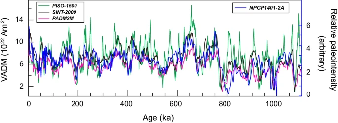
Wavelet-based verification of a relative paleointensity record from the North Pacific
Ji Young Shin, Yongjae Yu & Wonnyon Kim
Earth, Planets and Space volume 71, Article number: 88 (2019) Cite this article
Abstract
We present a relative paleointensity (RPI) record for the last ~ 1.1 Myr estimated from a sediment core in the central North Pacific, with quality verification using wavelet analysis. Rock magnetic analysis reveals that a stable remanence is carried mainly by single-domain (SD) biogenic magnetite and pseudo-SD detrital magnetite and that concentration- and grain-size-related bulk magnetic parameters vary by a factor of 3, initially meeting a conventional standard for RPI estimation. However, a further test using wavelet spectra of RPI proxies normalized by anhysteretic remanent magnetization (ARM) or isothermal remanent magnetization (IRM) shows intermittent orbital contamination at period of 100 kyr. A part of the 100-kyr orbital frequency in ARM-normalized RPI has a coherence and physical relationship with the normalizer. For the same time interval, a prominent 100-kyr cycle in the ARM/IRM wavelet spectra is also coherent with RPI, indicating that relative changes in biogenic and detrital magnetite were not well compensated by ARM normalization. For the selected RPI proxy using IRM normalization, a significant physical relationship with the lithology of magnetic minerals was not detected in the wavelet analysis, and thus, its intermittent orbital cycles could be of climatic origin, probably induced by non-magnetic factors. Nevertheless, our RPI record is consistent with global RPI stacks and provides a successful reconstruction of paleointensity with geomagnetic field origin in the North Pacific.
Introduction
Temporal variations in geomagnetic paleointensity are fundamental for understanding the geodynamo process and have therefore been closely investigated via geological materials such as rocks and sediments (e.g., Tric et al. 1992; Laj et al. 2000; Channell et al. 2014). In particular, relative paleointensity (RPI) values recorded in sedimentary sequences provide insights into the long-term variations in the geomagnetic field and show a global coherency over millennial timescales despite environmental differences and possible physical uncertainties of the recording process (e.g., Tauxe et al. 2006; Roberts et al. 2013). With increasing numbers of well-constrained long RPI records, time-varying paleointensity records have been integrated into global models, which now extended through the entire Quaternary (e.g., SINT-800: Guyodo and Valet 1999; SINT-2000: Valet et al. 2005; EPAPIS-3Ma: Yamazaki and Oda 2005; PISO-1500: Channell et al. 2009; PADM2M: Ziegler et al. 2011). Such globally stacked RPI data have a practical advantage in constraining sedimentary chronology, particularly for marine or lake environments that lack carbon or oxygen isotope dating (Roberts et al. 2013). However, high-quality RPI records from various geographic locations are still necessary to improve and evaluate the global models. In recent decades, few RPI records from the North Pacific (e.g., Kent and Opdyke 1977; Roberts et al. 1997; Yamazaki 1999) have contributed to the global stacks for the past 2 Myr, including SINT-2000 and PADM2M. These North Pacific RPIs, covering relatively short periods of geological time (< 0.9 Myr), are also insufficient for understanding the longer-term behavior of the geomagnetic field. Although a longer RPI record for the time interval of ~ 0.35–1.60 Ma has been documented (Yamazaki and Kanamatsu 2007), this record is not included in any of the global stacks.
Previous studies have discovered ~ 40-kyr or ~ 100-kyr cycles from the North Pacific RPI records, using spectral or wavelet analyses, suggesting orbital forcing of geomagnetic field variations (Kent and Opdyke 1977; Yamazaki 1999; Yokoyama and Yamazaki 2000; Yamazaki and Kanamatsu 2007; Yokoyama et al. 2007). Searches for orbital periods in paleointensity have also been performed for high-resolution and globally stacked RPI signals such as SINT-800, SINT-2000, and PISO-1500 (e.g., Heslop 2007; Channell et al. 2009), as well as deep-sea floor magnetization records and beryllium production records (e.g., Thouveny et al. 2008; Saracco et al. 2009). Some studies have suggested relationships between orbital signals and paleomagnetic intensity and directional changes (e.g., Fuller 2006; Thouveny et al. 2008), but no statistically significant orbital periods have been detected from global RPI stack records (e.g., Heslop 2007; Channell et al. 2009; Ziegler et al. 2011).
Xuan and Channell (2008) found that intermittent orbital cycles in some local RPI records are due to lithological or climatic contamination. Because the origin of such orbital cycles can be connected to lithological variations of magnetic minerals, the coherence between RPI and magnetic parameters including the normalizer used in RPI estimation has also been tested (e.g., Yamazaki and Kanamatsu 2007; Xuan and Channell 2008). In particular, in the case of marine sediments containing a mixture of biogenic and detrital magnetites, the different physical properties of these magnetites could result in coherence between RPI and the normalizer owing to incomplete normalization (Roberts et al. 2013), thereby complicating the record of paleointensity (Ouyang et al. 2014). However, such possible contamination of RPI from the two magnetite assemblages has not been fully assessed. The wavelet method is a useful way of detecting periodicities in non-stationary time series, including geomagnetic records (e.g., Guyodo et al. 2000; Heslop 2007; Xuan and Channell 2008; Channell et al. 2009), compared with power spectral analysis without time resolution. In addition, cross-wavelet analysis and wavelet coherence provide a powerful test for a physical link between two time series (Torrence and Compo 1998; Torrence and Webster 1999; Grinsted et al. 2004) and have been applied in investigating the presence of a phase relationship between RPI records and sedimentary lithologies (e.g., Guyodo et al. 2000; Xuan and Channell 2008). For example, Guyodo et al. (2000) were the first to analyze the cross-wavelet powers and phases of RPI versus rock magnetic records and proved a secondary lithological overprint on the RPI record.
Chromium6- Posts : 729
Join date : 2019-11-29
Miles Mathis' Charge Field :: Miles Mathis Charge Field :: The Charge Field Effects on Humans/Animals