
Possible Charged Particle Field
Page 14 of 15 •  1 ... 8 ... 13, 14, 15
 ![]()
Re: Possible Charged Particle Field
![]() by LongtimeAirman Mon Feb 18, 2019 10:00 pm
by LongtimeAirman Mon Feb 18, 2019 10:00 pm
I'll share my meager progress.
Jump right into overdrive. EQS406. With r=1 particles, the minimum spherical radius - without particle contact, is just under 14. At that distance, the r=1 particles are 8.35 angular degrees. Contact occurs between the 3 and the nine particle ring latitudes. Using equatorial offsets, we can add an equator and a new latitude ring. The original 8 equatorial latitude rings, (with 30,30,36,36,36,36,30,30 particles) separated by about 10 degrees have been replaced with 11 latitude rings (of 30 particles each) separated by 7.1916 degrees. N increased from 406 to 472. Not shown. That number could be increased further by addressing the pole latitudes, but I don’t see the point pushing past overdrive – that’s supposed to be our limit. It makes sense to start with a smaller EQS solution, with two less latitude rows compared with 406, then optimize that solution to replace the existing EQS406.
With that in mind I’ll begin with EQS372 northern hemisphere latitudes (up from the equator at zero) and particle ring counts.
[ 11.25, 12 ], // 30 particles
[ 22.5, 12 ], // 30 "
[ 33.75, 12 ], // 30 "
[ 45, 17.1429 ], // 21 "
[ 56.25, 20 ], // 18 "
[ 67.5, 24 ], // 15 "
[ 78.75, 40 ], // 9 "
[ 88.5, 120 ] // 3 "

Working the Overdrive EQS optimization.
Using equatorial offsets, of 360/30/2 degrees, I added a new 30 particle equatorial ring which bumped the EQS372 up to a modEQS402. With r=1 particles, the minimum spherical particle configuration radius - without particle contact, for the 372 (and 402) is just under 12, two smaller than the 406 radius, so the particles appear larger in the modEQS402 image.
I see the 402 is a good improvement in particle uniformity over the EQS406. I'll work the pole ends next, beginning with rotating the 3 particle pole rings by 20 degrees about the pole-to-pole axis. I'll move and may even might add a new polar latitude as well. All changes are straightforward. The particle count should increase a little bit more.
I'll be busy offline for the next two days.
.
LongtimeAirman- Admin
- Posts : 2026
Join date : 2014-08-10
Re: Possible Charged Particle Field
![]() by LongtimeAirman Thu Feb 21, 2019 5:59 pm
by LongtimeAirman Thu Feb 21, 2019 5:59 pm
EQS406 versus modEQS372.
Our simulated charge field particles react to the ambient charge field according to the ‘charge’ received at their charge sampling points. Those points are currently calculated by an equi-iso-latitudinal area algorithm called EQS. We currently use three EQS solutions - 46, 130 and 406.
Any algorithm has its purpose and limitations. We may improve the behavior of our charge field particles by increasing the uniformity of the sample point distribution sets over our current EQS precision ‘standards’ by careful modifications. We can conveniently display those sampling point distribution sets by placing neutral particles in the ‘same’ spherical configurations for easy review. These mods may indicate simple improvements to the algorithm itself.

EQS406 compared to EQS 342 modified into modEQS372.
Please reference the above image. In my last post I showed the ‘Overdrive’ spherical configuration - EQS406 and possible alternative configuration, modEQS402 still needing some pole optimization. That pole mod led me to begin at a different EQS solution, modifying EQS342 into a modEQS372, currently my recommended replacement for EQS406.
As in my previous post, with r=1 particles, the minimum spherical particle configuration radius without particle contact, for the EQS342 (and modEQS372) is just under 12. The ‘minimum’ EQS406 radius without particle contact is 14. The EQS406 has 9 northern hemisphere latitude particle rings separated by about 10 degrees: (3, 9, 15, 20, 24, 30, 30, 36, 36). That same set is repeated in the southern hemisphere.
Starting with EQS342 - (3, 9, 15, 18, 21, 30, 30, 30, 30, 30, 30, 21, 18, 15, 9, 3). Sixteen latitude rings, totaling 342 points. Make the following modifications:
1. Adding single particles over the poles. EQS doesn’t provide single pole particles. [ 90, 360 ] results in a particle that ‘leans’ on the p-to-p axis.
2. Offsetting adjacent pole latitude rings. EQS partitions the spherical surface in both latitude and longitudinal alignments. Instead of the current six minimum gaps; point the hex between 2 of the 12 particles in the next particle ring instead of directly at six of them by rotating the 6 particle ring latitude 360/12/2 or 15 degrees. If the pole was three point, it would need the same rotation with respect to its neighboring latitude. Pole latitudes numbers that aren't evenly divisible may not benifit from offset rotations. Note, the modEQS372 in the image still needs its hex rotation. EQS342’s polar latitude group: 3, 9, 15, 18, 21 was changed to modEQS372’s 1, 6, 12, 18, 21, 24.
3. Offsetting adjacent equatorial latitude rings. Given rows of equal number (30) particle rings, we can increase the distance between adjacent (elevation) particles by alternating the starting positions of the each particle ring 360/30/2, 6 degrees. Offsetting adjacent latitudes allows us to change reduce the elevation angle of adjacent latitudes results the resulting distinctive hexagonal alignments.
4. Adding a new 30 particle ring over the equator. Note, all EQS algorithm solutions lack equatorial rings. Offsetting the equatorial latitudes has allowed us to replace the previous 6 latitudes with 10 degree separation to 7 latitudes, each separated by 8.7 degrees, with resulting distinctive hexagonal alignments.
The result is modEQS372 - (1, 6, 12, 18, 21, 24, 30, 30, 30, 30, 30, 30, 30, 24, 21, 18, 12, 6, 1). 19 latitudes with 372 points. The modifications above result in increased numbers of particles at EQS342’s radius of 12, without allowing r=1 particles to overlap; EQS406’s minimum radius without r=1 particle overlap is 14.
The new modified distribution is densest between adjacent (azimuthal) particles within the two +/-30 particle ring latitudes at the shoulders. The ‘density’ of points reduces toward both the equator and poles.
The main limitation of this method is maximizing the number of equal particle ring latitudes. I believe there are just a small set of two modifiable EQS solutions at this ‘scale’, involving only those solutions with 4 or 6 equal particle length equatorial latitudes. ModEQS372 handles the 6 case, six equatorial latitudes become the modified seven. The EQS130 competition will handle the other, by changing an EQS solution with 4 adjacent (elevation) equal particle equatorial latitudes into the modified five.
EQS130 contenders next.
.
Last edited by LongtimeAirman on Thu Feb 21, 2019 7:00 pm; edited 1 time in total (Reason for editing : Typos!)
LongtimeAirman- Admin
- Posts : 2026
Join date : 2014-08-10
Re: Possible Charged Particle Field
![]() by LongtimeAirman Sat Feb 23, 2019 12:14 pm
by LongtimeAirman Sat Feb 23, 2019 12:14 pm

EQS130, along with two alternatives, modEQS128 and modEQS144 are shown. A few small changes to the existing EQS algorithm (ex. EQS 130) result in the two modified and, I believe, improved (equidistant) point distributions - as shown.
You have my sympathies, post after post of particles in spherical configurations. This is a working project and the devil’s in the details. As you no doubt already know (too well), the present goal is to improve the uniformity of distribution (equi-distance wise) of our calculated particle’s charge field sampling points. That should have the side benefit of improved overall performance of our possible charged particle field simulation engine.
Note that the engine is being used as a tool to model the sampling points of a single particle as particle configurations. Aside from my autocad modifications, our particle engine allows one to make these models. I consider them as real and valid in some sense, although to be perfectly honest, I cannot explain nor justify the validity of spherical particle configurations with respect to the charge field. Nevertheless, I’ll work toward developing a spherical group UI that will allow a casual user to create many of them herself. Then that single spherical UI scenario could allow me to discard several redundant and tool scenarios currently in the Spherical group.
The user just selects from these precision levels: Low, Med, High and Overdrive. The default is low. I discussed Overdrive in my last post. EQS130 is our simulation’s high Precision standard, made up of (3, 9, 15, 18, 20, 20, 18, 15, 9, 3), 10 particle ring latitudes totaling 130 particles, and is shown in the top row of the image. This configuration begins to overlap the r=1 particles at about R=7.1. R=7.5 in the EQS130 first row of images.
ModEQS128. – (1, 6, 12, 18, 18, 18, 18, 18, 12, 6, 1), 11 rings, 128 particles. The first alternative to ECP130 begins with EQS108 – (6, 12, 18, 18, 18, 18, 12, 6), 10 particle ring latitudes totaling 108 particles. The configuration begins to overlap the r=1 surface particles near R=6.6. R=7 in the EQS108, as well as the modEQS128– second row images. The modifications are as follows:
1. Add single pole particles.
2. Rotate the 6 particle ring pole, 360/12/2 = 15 degrees. This allows slightly more room between the 6 and 12 particle ring latitudes – say for a slightly larger 6, or smaller 12 particle rings.
3. Convert the four equatorial 18 particle rings into five by adding a new 18 particle ring and
4. Offsetting, or alternating the starting point of each adjacent 18 particle latitude ring by 360/18/2 = 10 degrees (az) so that the 5 rows will form a hexagonal pattern.
ModEQS144 – (3, 9, 15, 18, 18, 18, 18, 18, 15, 9, 3), 11 rings, 144 particles. It is also shown (third row) at the configuration radius R=7. It began as EQS126 (3, 9, 15, 18, 18, 18, 18, 15, 9, 3). Here are the 144 modifications:
1. Rotate the pole triangles 360/9/2 = 20 degrees (az).
2. Offset equal particle (18) equatorial latitudes 360/18/2 = 10 degrees, thereby making room to;
3. Add a new 18 particle latitude ring, increasing the number equatorial latitudes from 4 to 5 in the same area.
I believe both the ModEQS128 and ModEQS144 alternatives provide more uniform point distributions then EQS130.
I’ll look at EQS46, the Medium Precision, next.
.
LongtimeAirman- Admin
- Posts : 2026
Join date : 2014-08-10
Re: Possible Charged Particle Field
![]() by Nevyn Thu Mar 07, 2019 12:57 am
by Nevyn Thu Mar 07, 2019 12:57 am

Nevyn- Admin
- Posts : 1887
Join date : 2014-09-11
Location : Australia -

Re: Possible Charged Particle Field
![]() by LongtimeAirman Thu Mar 07, 2019 2:29 pm
by LongtimeAirman Thu Mar 07, 2019 2:29 pm
I don’t see how the methodology I’ve been using can “optimize” the EQS46. I suppose I could come up with an objective quantitative measure of equi-spaced points in order to evaluate the EQS46, and then compare it to an alternative, there are many standard polyhedral forms to choose from. I also wanted to give an additional look at the geodesics. Also I’m sure the ‘fullerene’ icosa-based carbon configuration, C60 would be better choice than the EQS46.
Here’s another idea I’ve picked up in my readings, that I need to pass by you. Particle placements based on repulsion; our possible charged particle field should be able to handle that. Using the EQP algorithm, an arbitrary number of Protons can be positioned at the spherical configuration’s radius with their south poles oriented toward the spherical configuration’s center. I imagine the protons’ emission fields may then push each proton into optimal positions which we may then use as an ideal Precision solution set for that number of points.
In order to do that, we must constrain the protons’ motions to the spherical radius. Specifically, is it possible - relatively easily – to: 1. Immobilize, fix, or make Unmoveable - both the proton’s spin axis to always point to the configuration center; as well as 2. Fix the protons distance from that center?
Optimistic, eh? I had to ask.
.
LongtimeAirman- Admin
- Posts : 2026
Join date : 2014-08-10
Re: Possible Charged Particle Field
![]() by Nevyn Thu Mar 07, 2019 5:27 pm
by Nevyn Thu Mar 07, 2019 5:27 pm
In order to test the charge point configurations, we can use a bit of math. There is probably some better way to do it, but when I'm in unknown territory and can't see a nice solution, I tend to brute force it and then look for optimizations later.
We take each generated charge point and we calculate the distance to all other particles. We then find the minimum value from that set. So we end up with a minimum value per charge point. Then we compare all of the minimum values to each other. There are many ways to do that but just putting them into a graph would be a good start. If you end up with a straight horizontal line, then you have found an optimal solution. The most optimal solution is that which is closest to Y=0 on the graph.
Nevyn- Admin
- Posts : 1887
Join date : 2014-09-11
Location : Australia -
Re: Possible Charged Particle Field
![]() by LongtimeAirman Fri Mar 08, 2019 10:21 pm
by LongtimeAirman Fri Mar 08, 2019 10:21 pm
Airman. Ok, nix the repulsion idea.Nevyn wrote: Yes, those things are possible, but it isn't pretty and breaks the model we are trying to create. … .
With respect to points on a sphere, I believe repulsion is actually an iterative process. Based on increasing the distance between the closest points in the set of N points on a sphere at a given iteration. It’s another possible alternative to our current EQS and EQP algorithms I hadn’t gotten into - there are many. Equi-distant points on a sphere aren't true beyond the platonic solids, and are only approximated. I thought if we had ‘real proton repulsion’ - given an EQP starting set – it might work; but you’re correct, I ‘overlooked’ the constant motion of the non-zero velocities as the protons keep repelling each other.
I should point out my obvious thinking. Fixing orientations and distances in the way I suggested mimics the coherence orientation. I suppose any coherence in our possible charged particle field would also require a custom model.
I take it you would like to see some quantitative measure in support of selecting alternative precision candidates, suggesting “brute force” for a start. That’s a change, up to now, I’ve been relying on images to compare the precision candidates, I’ll shoot for numbers too.Nevyn wrote: In order to test the charge point configurations. ...
We take each generated charge point and we calculate the distance to all other particles. …
With that in mind, and not for the first time, I googled something like “equi-spacing points on a sphere”, and found an algorithm based on s-curves on the sphere. It’s undergraduate, easy to read for anyone interested in the subject. Nice looking results and it also includes an efficiency function that sounds like what you had in mind.
A New Computationally Efficient Method for Spacing n Points on a Sphere Jonathan Kogan https://scholar.rose-hulman.edu/rhumj/vol18/iss2/5/
Pages 54 – 71.
Pg 62. … we first created three new functions to analyze how well the points were spaced on a sphere: SmallestDistance, TheoreticalSmallestDistance, and NormalizedSmallestDistance.
SmallestDistance(pts) takes a list of points and identifies the smallest Euclidean distance between any two points on the sphere. In other words, it identifies the two points that are closest together and outputs the distance between the two.
The TheoreticalSmallestDistance(n) function returns the upper bound for the distance of n equally spaced points on a sphere. It is well known that the optimal spacing of points on the plane is the hexagonal grid. To find the upper bound for the distance of n points on a sphere, we imagine there is a planar hexagonal grid that covers the entire area of the sphere. Using this grid, we find this upper bound for all n values based on the size and the number of equilateral triangles.
Lastly, we defined the NormalizedSmallestDistance(pts) function as the SmallestDistance(pts)/TheoreticalSmallestDistance(Length(pts)); the function provides a relative accuracy for the points that are around the sphere.
Also, the results look good. The Mathematica code is included, here's the Python code.
Pg 70. The research discussed in this paper has also led to the creation of the Mathematica function SpherePoints[n], which was added in the Mathematica 11.1 update [10]. This Mathematica function enables anybody who wants points spaced equally on a sphere to generate them quickly and easily [8].
- Code:
Pg 72. A.2 Python Code

import math
def spherical coordinate (x , y ):
     return [math. cos (x) ∗ math. cos (y) ,
     math. sin (x) ∗ math. cos (y) , math. sin (y )]
def NX(n, x ):
     pts =[]
     start = (−1. + 1. / (n − 1.))
     increment = (2. − 2. / (n − 1.)) / (n − 1.)
     for j in xrange(0 , n):
           s = start + j ∗ increment
          pts . append(
          spherical coordinate (
          s ∗ x , math. pi / 2. ∗
          math. copysign (1 , s ) ∗
          (1. − math. sqrt (1. − abs( s )))
          ))
     return pts
def generate points (n):
     return NX(n, 0.1 + 1.2 ∗ n)
LongtimeAirman- Admin
- Posts : 2026
Join date : 2014-08-10
Re: Possible Charged Particle Field
![]() by LongtimeAirman Fri Mar 15, 2019 6:31 pm
by LongtimeAirman Fri Mar 15, 2019 6:31 pm
Status update. Unfortunately, Jonathan Kogan’s paper didn’t provide all the details. The program is more complicated than it first appeared, and I haven’t decided how I should go about re-organizing the code I previously posted. The important thing is supposed to be the “efficiency measure”. Requoting TheoreticalSmallestDistance(n), “we imagine there is a planar hexagonal grid that covers the entire area of the sphere”, that’s all the information provided on that subject.
I decided to go through the exercise of figuring out the efficiency measure while adding a simpler type of spiral algorithm, based on the Golden ratio. From, Evenly distributed points on sphere,
https://web.archive.org/web/20060728050730/http://cgafaq.info/wiki/Evenly_Distributed_Points_On_Sphere. Also Points on a sphere, October 4th, 2006 by Patrick Boucher. //http://www.softimageblog.com/archives/115
- Code:
     inc := pi*(3-sqrt(5))
     off := 1/(2*N) - 1
     for k := 0 .. N-1
            z := k/N + off
            r := sqrt(1-z*z)
            phi := k*inc
            pt[k] := (cos(phi)*r, sin(phi)*r, z)
In the meantime, I found Jonathan Kogan’s youtube video of his paper, A New Computationally Efficient Method for Spacing n Points on a Sphere
.
The Efficiency measure, including the TheoreticalSmallestDistance(n) equation I was searching for appears to be part of a small set (3 or 4(?)) of slides – not included in the paper - that served for brief glimpses in the two videos, good enough for a screen capture.
- Code:
smallestDistance[pts_] := min[table[N[euclideanDistance[pts[[i]], pts[[j]]]],{i,1.0, length[pts]}, {j, i + 1.0, length[pts]}]]
 theorecticalSmallestDistance[pts_] := Math.sqrt(8*Math.PI/(n*Math.sqrt(3)))
 normalizedSmallestDistance[pts_]:= smallestDistance[pts]/theorecticalsmallestDistance[length[pts_]]

Outputs for the new Golden ratio spherical algorithm with Efficiency measure are shown. Above, the spherical configuration GS50 is on the left and GS406 (from the inside) is on the right. We are looking down along the main N/S y axis for both. While the overall spacing is nice, the poles are either clumped or open.
The Efficiency Measure for GS406 is shown below. Assuming I implemented it correctly the normalized efficiency measure is a poor 0.674. According to Kogan’s paper the best efficiences are about 0.85. Radius 16 is cutting it close, the two closest r=1 neutrons are separated by just 0.040 – almost touching. If one were interested in the just the efficiency numbers, it’s easy to switch between the Parameters and Output control tabs. Curious to see the results, beginning with 10, and incrementing by five up to 65, then 130, then 406, the best efficiency I found was 0.7115 for 10 neutrons, with a fairly straight line dropping to the the GS406’s 0.674. The Golden ratio I implemented is not a good source for equi-distant spaced points necessary for our desired charge detection Precision candidates.

.
Last edited by LongtimeAirman on Fri Mar 15, 2019 7:05 pm; edited 1 time in total (Reason for editing : Added efficiency code)
LongtimeAirman- Admin
- Posts : 2026
Join date : 2014-08-10
Re: Possible Charged Particle Field
![]() by LongtimeAirman Wed Apr 10, 2019 1:22 pm
by LongtimeAirman Wed Apr 10, 2019 1:22 pm

Kogan spiral algorithm, 201 r=1 Neutrons, the configuration radius is 25.
The Kogan spiral algorithm and efficiency measure has been added to the spherical scenarios. Now that we have pictures as well as numbers we can make actual qualitative comparisons. Here’s an abbreviated efficiency calculation - Smallest/Theoretical - for the current three EQS precision standards versus EQP, Golden and Kogan algorithm results.

EQP with 404 particles at 0.797 is higher - better point distribution efficiency - than EQS 406 at 0.788 and Kogan 406 at 0.789.
Next, if I continue as planned, I should look at modifying EQS results by adding an equatorial row of particles and rotating alternate latitudes which could improve the current EQS standard. Also, as I mentioned previously, I should be getting better Golden results. I need to look into that too.
.
LongtimeAirman- Admin
- Posts : 2026
Join date : 2014-08-10
Re: Possible Charged Particle Field
![]() by LongtimeAirman Thu Apr 18, 2019 9:53 pm
by LongtimeAirman Thu Apr 18, 2019 9:53 pm

Well Sir, great pain and joy, another fine possible charge particle engine programming tasking is tentatively complete, an efficiency measure is now included with most all our point configurations. Assuming it’s correct, the expanded efficiency table above shows the results.
The polyhedral vertex set – octahedron, cube, icosahedron and pentagonal dodecahedron surprised me. I had assumed the platonic solids were the only ideal solutions. The equidistant spacing of the vertices of the octahedron are the most ideal on the board - 0.908 - closest to one. What does the icosa’s greater than one value, 1.119 mean? Mediocre cube and dodeca values. I can see why the hoso’s are extinct.
The EQS precision set: 46, 130 and 406 are bold and highlighted. EQS238-0.846, and EQS312 – 0.849, would make better standards than EQS 130 and 406. I apologize for giving you grief over the rectangular plot algorithm which you converted to centroids. Given it’s overall values, I have a greater respect for the EQS algorithm and your implementation of it.

I claimed I could improve the efficiencies of some EQS solutions by adding an equatorial particle ring, or pole particles, rotating alternate equatorial or polar latitude rings, so I created a new spherical group scenario “EQS Mods” that shows such mods to EQS336: The result is a very respectable Mod EQS374 with efficiency value of 0.838. I didn’t quite follow the ‘dw centroids logic’ so I adjusted the latitudes by eye, trial and error. I need to work this with autocad and see if I can improve that number further.
Once again, the Golden algorithm has a poor and very linear efficiency result – it must be wrong. On the other hand, the new Kogan algorithm is as good as Golden. K201 or K326 would make fine standards.
The primary benefit of this table is that it provides sufficient justification in selecting a more efficient short list of precision alternatives.
Any thoughts? Feedback? Additional taskings?
.
LongtimeAirman- Admin
- Posts : 2026
Join date : 2014-08-10
Re: Possible Charged Particle Field
![]() by Nevyn Sat Apr 20, 2019 1:05 am
by Nevyn Sat Apr 20, 2019 1:05 am
I spent a bit of time implementing a way to test the algorithms. I've pushed some new changes to do so, but there is no code that uses it yet. Here is what I have implemented:
Statistics of Points representing the Surface of a Sphere
We have some algorithms that generate points on the surface of a sphere, and we want to find the most even representation of that surface. We want each point to be of equal distance to its neighbours. In order to evaluate these algrithms, we must gather statistics about the data they generate.
In the first instance, our data is a series of points. We want to know how far each point is from all other points. For each point in the data set, we calculate the min, max, average and range of the distance to all other points. That gives us an array of min values, one for each point, and an array of max values, etc, etc.
That brings us to the second instance where we have a new data set containing statistics for each location generated by an algorithm. Statistics are addictive, you can't have just one, so let's gather some more statistics from the statistics that we already have.
Now we are analyzing each data set in isolation to the others. We are calculating the min, max, average and range of all mins, then all max values, then all averages and finally, all of the ranges. In the end, we reduce it all down to 16 numbers. Most of which are useless, but we'll get to that in a minute. This is what our final data set looks like:
- Code:
{
  min: {
    min: <number>,
 max: <number>,
 avg: <number>,
 range: <number>
  },
  max: {
    min: <number>,
 max: <number>,
 avg: <number>,
 range: <number>
  },
  avg: {
    min: <number>,
 max: <number>,
 avg: <number>,
 range: <number>
  },
  range: {
    min: <number>,
 max: <number>,
 avg: <number>,
 range: <number>
  }
}
Now we need to figure out which values mean something to this problem and help us to determine which is the better algorithm. Let's look at each data set and see what it is telling us.
Minimums:
The min data set can tell us how much deviation there is from true equality between points. This is a critical data set for this problem, as it represents the data we are trying to minimize between algorithms. Of particular interest is the range, which we want to approach zero. An algorithm that reached zero would have true equal distance between all points.
The min.min value represents the closest of all point pairs. This value ultimately comes from only 2 points in the original data set.
The min.max value represents the largest minimum of all point pairs. Same as with the min, only 2 points are used to calculate that value. This is the worst that the algorithm gets. Minimizing this value is important. We want min.min and min.max to approach each other.
The min.avg value represents the average minimum distance between points and gives us a general representation of an algorithm. This is probably a good value to initially look at to gauge algorithms. If you have to represent an algorithm with a single value, this is the one to use. While not exactly as important as others, it gives the best general idea of how an algorithm will perform.
Note that the min.avg value, and indeed all values really, heavily relies on the radius used. You must choose one radius and use it for all algorithms in order to be able to compare the numbers. A unit radius is generally the best.
The min.range value represents the difference between the smallest minimum and the largest minimum, therefore, it is a very important value. The closer this is to zero the better.
Maximums:
The max data set can tell us how balanced the points are on the sphere. In a truely balanced set of points, every point has an equal and opposite point from it. The line between those 2 points goes through the center of the sphere. The maximum value for any given point represents the point that is farthest from it. If that value equals the diameter of the sphere, then balance is achieved. If max.range also equals zero, then every point has an opposite.
This is not of important interest, and would not be used to differentiate algoithms in the first instance. If you have a few algorithms that appear equal, then this kind of balance may be used to differentiate them and choose a winner.
The max.min value represents the smallest maximum value.
The max.max value represents the largest maximum value.
The max.avg value represents the average maximum value.
The max.range value represents the difference between the largest maximum value and the smallest maximum value.
If max.avg equals the diameter and max.range equals zero then true balance is achieved.
Average:
The avg data set is of little use, but can be used like the max data set to determine balance. Since it is more dangerous to use as such, it can be ignored for this problem.
The avg.min value represents the smallest average value.
The avg.max value represents the largest average value.
The avg.avg value represents the average average value. Does that even mean something? I think we've gone too meta.
The avg.range value represents the difference between the largest average value and the smallest average value. It can be used to determine increasing uniformity as it approaches zero.
Range:
The range data set is not very important.
The range.min value represents the smallest range value.
The range.max value represents the largest range value.
The range.avg value represents the average range value. A good indicator of uniformity. The closer to zero the better.
The range.range value represents the difference between the largest range value and the smallest range value.
To analyze a set of algorithms, we calculate these values for each algorithm, using the same radius, and then put the important values into a table. Look at those values and see which algorithms look the best.
I have implemented a few new methods in the LocationCreator class to generate these statistics. I've even created a little helper method to just return the important ones, which are only 6 values out of 16. You need to implement each of the algorithms as a LocationCreator, just like you have with EQP. I suggest you copy the eqp.js file to a new file for each new algorithm, renaming each like algorithm-name.js, just like eqp.js and eqs.js, etc.
I'll look into creating a new modal dialog that will calculate the stats and present the results for all known algorithms in a table.
Nevyn- Admin
- Posts : 1887
Join date : 2014-09-11
Location : Australia -
Re: Possible Charged Particle Field
![]() by Nevyn Sat Apr 20, 2019 3:25 am
by Nevyn Sat Apr 20, 2019 3:25 am
It shows your EQP improvements are very close to the standard EQS algorithm. I'm not sure what they look like, but the numbers look good. I created 3 versions to match the EQS variants. I'm not sure if they are good values or not. Have a look at the bottom of eqs.js to see what I did there. Play around with the numbers to try different options.
Nevyn- Admin
- Posts : 1887
Join date : 2014-09-11
Location : Australia -
Re: Possible Charged Particle Field
![]() by LongtimeAirman Sat Apr 20, 2019 1:30 pm
by LongtimeAirman Sat Apr 20, 2019 1:30 pm
Nevyn wrote. I'm not sure how you are calculating those numbers. What equation are you using?
Airman. The efficiency measure numbers I’ve shown in my tables are the normalizedSmallestDistance[pts_].
normalizedSmallestDistance[pts_]:= smallestDistance[pts]/theoreticalsmallestDistance[length[pts_]]
var smallestDistance = minimum;
The only measured value is the smallestDistance, what you referred to as min-min.
var theoreticalSmallestDistance = radius * Math.sqrt((8*Math.PI)/((n)*(Math.sqrt(3))));
The theoreticalSmallestDistance provides an ideal value for any radius and number of particles. Please consider including it in your statistical set. It allows a way to measure across configuration sets – at a given radius and number of particles – as Kogan mentions in his paper.
Nevyn wrote. It shows your EQP improvements are very close to the standard EQS algorithm. I'm not sure what they look like, but the numbers look good. I created 3 versions to match the EQS variants. I'm not sure if they are good values or not. Have a look at the bottom of eqs.js to see what I did there. Play around with the numbers to try different options.
Airman. We have a disconnect. I’ve made no EQP improvements. I added the EQP set to the particle engine’s precision set two months ago. I added the above efficiency measure to the spherical group scenario EQP Points last month. I should point out, when one selects the ‘approximate number’ of EQP particles of 406 in the parameter tab, here’s the calculated output table:
Only 404 particles.404 Neutrons. The configuration radius is 17.1. The smallest distance - between the centers of the two closest particles - is 2.581, between neutrons 1 and 2. The theoretical distance is 3.241. Smallest/Theoretical is 0.797.
Since that time, I’ve included the same efficiency measure in all the spherical configurations on their Output control tabs. My latest effort over the last day or two has been in trying to understand EQS var cellAngles well enough to modify it by adding new latitudes. To be honest, I want to throw out the angle and lastAngle averaging and list the desired particle latitudes directly, but that would be changing your centroid calculation.
In case of confusion; I had to give a quick reply lest you be working under a false assumption. I appreciate the stat breakdown and enthusiasm. I'd be happy to include any additional info on the user side of the firewall, on the output control tab’s output table if at all possible.
P.S. Added two same "and number of particles" as in; The theoreticalSmallestDistance provides an ideal value for any radius and number of particles.
.
Last edited by LongtimeAirman on Sat Apr 20, 2019 2:29 pm; edited 2 times in total (Reason for editing : Added P.S.)
LongtimeAirman- Admin
- Posts : 2026
Join date : 2014-08-10
Re: Possible Charged Particle Field
![]() by Nevyn Sat Apr 20, 2019 9:32 pm
by Nevyn Sat Apr 20, 2019 9:32 pm
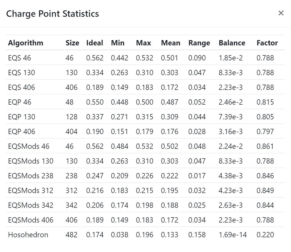
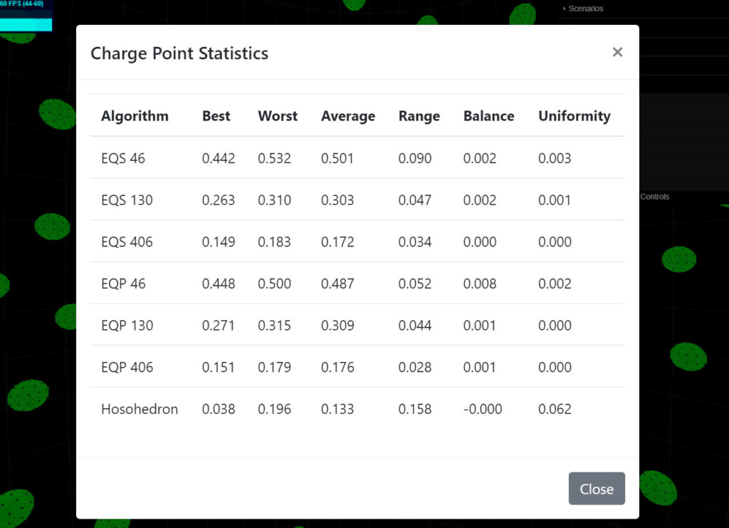
I combined the Balance and Uniformity fields together (and also changed the value being used for the uniformity), because I was out of space. Added in the sample size to show the actual number of points used. The Ideal column shows the theoretical smallest distance, using your equation. I haven't read up on it, so I don't know if it applies to all situations or just whatever Kogan was working on in that paper. The EQS algorithm beats it, though, so it seems to be limited.
I put the Ideal value right next to the Min and Max values, because that is what we want to compare it against. The last column, Factor, is Min/Ideal. I used the Min at first, but it didn't really work. I tried the Average and the results looked better to me. That is the average of the minimum values, so it represents all minimums rather than just the best minimum.
Here is the table using Average/Ideal:

We want to find an algorithm that has a low Range and Balance, and a Factor close to 1. The EQS algorithm is still looking the best to me. You're right about EQP, it isn't complete, but it does have some different cell angles being used. EQSMods is a new one where I extracted the cell angles from your spherical.js scenario, but then realised that the algorithm is different too, so it uses the angles, but not the new algorithm, just the standard EQS one.
Nevyn- Admin
- Posts : 1887
Join date : 2014-09-11
Location : Australia -
Re: Possible Charged Particle Field
![]() by LongtimeAirman Sat Apr 20, 2019 9:57 pm
by LongtimeAirman Sat Apr 20, 2019 9:57 pm
LongtimeAirman- Admin
- Posts : 2026
Join date : 2014-08-10
Re: Possible Charged Particle Field
![]() by Nevyn Sat Apr 20, 2019 10:56 pm
by Nevyn Sat Apr 20, 2019 10:56 pm
I'm using a radius of 1, so it falls out. That is what you are referring to as the theoretical value. The Factor column contains first the smallest/theoretical, then the average smallest/theoretical in the second pic.
Nevyn- Admin
- Posts : 1887
Join date : 2014-09-11
Location : Australia -
Re: Possible Charged Particle Field
![]() by Nevyn Sun Apr 21, 2019 6:04 pm
by Nevyn Sun Apr 21, 2019 6:04 pm

I have also used it as the Charge Point algorithm.

Not sure if it is better or not, but it looks cool.
Nevyn- Admin
- Posts : 1887
Join date : 2014-09-11
Location : Australia -
Re: Possible Charged Particle Field
![]() by LongtimeAirman Mon Apr 22, 2019 2:31 pm
by LongtimeAirman Mon Apr 22, 2019 2:31 pm
Agreed. I think the Kogan spiral algorithm is prettier and provides numbers close to the equi-latitudinal/longitudinal area solutions of the EQS or EQP algorithms.Not sure if it is better or not, but it looks cool.
With respect to precision alternatives, do we want to compare precision alternatives or do we want to provide a range of precision values? I favor the latter. Doing a quick review, I see the following current precision alternatives:
1. Low; 8 cardinal points octahedron;
2. Medium (K46);
3. High (K130);
4. Overdrive (K406);
5. EQP Medium (EQP46);
6. EQP High (EQP130); and
7. EQP Overdrive (EQP406).
In order to improve the range of our precision set consider:
EQP: We have EQP48 vice EQS46, EQP128 vice EQP130, and EQP404 vice EQP406 – none of the three EQP numbers agree with the EQS numbers to do a direct comparison, still, EQP128 may be slightly better than EQS13. More importantly, there doesn’t seem to be any good spherical alternatives between EQP46 and K201. So keep EQP128;
EQS: Keep EQS46, but drop EQS130. Add EQS 238 and/or EQS312. EQS406 has a low performance. The only alternative with a better performance near that number of particles would be my ModEQS374.
Kogan: Keep K46, but drop K130 and K406. Add K201 and K326.
That would make my proposed precision list:
1. Low; 8 cardinal points octahedron;
2. EQS46;
3. EQP128;
4. K201;
5. EQS238;
6. EQS312;
7. K326; and
8. ModEQS376;
.
LongtimeAirman- Admin
- Posts : 2026
Join date : 2014-08-10
Re: Possible Charged Particle Field
![]() by Nevyn Mon Apr 22, 2019 6:29 pm
by Nevyn Mon Apr 22, 2019 6:29 pm
There are still some issues at the poles. Not quite as bad as EQS and no where near as bad as most algorithms, but it is still there.
Nevyn- Admin
- Posts : 1887
Join date : 2014-09-11
Location : Australia -
Re: Possible Charged Particle Field
![]() by LongtimeAirman Mon Apr 22, 2019 9:15 pm
by LongtimeAirman Mon Apr 22, 2019 9:15 pm
You're the boss, I try to be self-motivating, but at the moment, I need directions.
If you agree, I'll load all the additional stats you've included with the new Statistics button in all the spherical scenarios Output control tab's Output table. That will enable us to collect the same data for every n of every spherical algorithm for direct comparison.
Feel free to direct or task me otherwise.
.
LongtimeAirman- Admin
- Posts : 2026
Join date : 2014-08-10
Re: Possible Charged Particle Field
![]() by Nevyn Wed Apr 24, 2019 12:37 am
by Nevyn Wed Apr 24, 2019 12:37 am
Nevyn- Admin
- Posts : 1887
Join date : 2014-09-11
Location : Australia -
Re: Possible Charged Particle Field
![]() by LongtimeAirman Wed Apr 24, 2019 6:40 pm
by LongtimeAirman Wed Apr 24, 2019 6:40 pm
Thanks for calling me off, but a few changes are necessary. Such as conforming my prior efficiency verbiage to agree with the new statistics data.You can add it to those scenarios if you want, but it will be easier to create another button ... .
The Charge Point Statistics button includes 9 items: Algorithm, Size, Ideal, Min, Max, Mean, Range, Balance, and Factor. In order to match the Statistics button output, the spherical scenarios efficiency calculations would need to rename four variables and add four new output variables: Max, Mean, Range, and Balance. So, thanks for clarification, other than changing names, I won’t be adding new values at present.
Still, I made good progress - for me. Working with point sets are fun. Each algorithm had its own set of efficiency calculations. I replaced those instances with function calls to a single instance; function calcStats( num, radius, xPts, yPts, zPts ). I changed most all the verbiage to agree with the Statistics button. Now, if you give the word, I can work on adding or changing all the spherical scenario Output tables in one place. I’ll push the change in a few hours.
Next, each algorithm has two instances of point set creations, for both statistics and particle placement. I suppose I should reduce that to just one functional point creation instance and two function calls (for each algorithm). It adds up.
.
LongtimeAirman- Admin
- Posts : 2026
Join date : 2014-08-10
Re: Possible Charged Particle Field
![]() by LongtimeAirman Thu Apr 25, 2019 8:01 pm
by LongtimeAirman Thu Apr 25, 2019 8:01 pm
Maybe we can plot the Kogan values off of the list you’re generating with the Statistics2 button?
Good progress today, I'll push the changes in a couple of hours. As hoped, I successfully converted the two instances of code creating point sets within each algorithm – for particle placement or distribution calculations – into two function calls, and one instance of function coding. I also corrected a problem with Poly points and calcStats that I pushed yesterday.
All the spherical configuration scenarios are now better organized. For example, it occurs to me I should create a single scenario where I can output any spherical set, just provide the desired: typeAlgorithm, number of surface particles, and configuration radius. Or I can put two or more configurations on the screen at once.
.
LongtimeAirman- Admin
- Posts : 2026
Join date : 2014-08-10
Re: Possible Charged Particle Field
![]() by LongtimeAirman Sun Apr 28, 2019 1:26 pm
by LongtimeAirman Sun Apr 28, 2019 1:26 pm
Currently, all the spherical configuration scenario’s surface particles share the same orientation - they are all aligned with the world coordinates. Turn on the Boundary and Particle axes graphics to see that all particle axes: n/s (y-axis, green), e/w (x-axis, red) and f/b (z-axis, blue), are parallel. I want to re-orient/rotate all the surface particles such that their n/s axis is pointed to the configuration center – the (0,0,0) position. The particles would then be aligned to the spherical configuration instead of the world. By adding a checkbox, the user can choose to align the particles one way or the other.

Each particle has a different, but not correct, orientation.
Of course, reorienting each particle properly is easier said than done. Adding insult to injury, quaternions are built into three.js, but I haven’t figured out how to make them work for this problem yet. The image above shows EQP46 particles improperly reoriented by this codeline –
var q = new THREE.Quaternion().setFromAxisAngle( new THREE.Vector3( points[i].x, points[i].y, points[i].z ), angle*i ); // angle = 2PIRad/number of particles.
I believe I need to do three cross products between each position and each axis. Then follow that up with three dot products to determine the angles. I’ve suffered this problem long enough to seek help. Here are two recent finds I must share:
Rotation Quaternions, and How to Use Them, by D. Rose - May, 2015. Short and straightforward, this paper includes a three step quaternion rotation process. Step 1: Convert the point to be rotated into a quaternion by assigning the point's coordinates as the quaternion's imaginary components, … . Step 2: Perform the rotation. … . Step 3: Extract the rotated coordinates from p'. ... .
3d Math Primer for Graphics and Game Development, Fletcher Dunn and Ian Parberry – 2nd edition, 2011. A wonderful ‘basics’ math book that I’ve always wanted. All you need - including physics - to create your own particle engine. As I understand it, this is a free e-book, in pdf, or you may choose to purchase a printed copy. Check it out.
.
LongtimeAirman- Admin
- Posts : 2026
Join date : 2014-08-10
Re: Possible Charged Particle Field
![]() by Nevyn Sun Apr 28, 2019 6:39 pm
by Nevyn Sun Apr 28, 2019 6:39 pm
Let:
p1 = center point of object
p2 = point to look towards
- Code:
// create a vector to represent the line from p1 to the point on the object that needs to be oriented towards p2
// I think this will be the Y axis for you
var align = new THREE.Vector3( 0, 1, 0 );
// calculate the vector between the location of the object and the target point
// this is where align will end up at the end of this algorithm
var v = new THREE.Vector3().subVectors( p1, p2 );
// calculate the angle between those 2 vectors
var angle = align.angleTo( v );
// calculate axis to rotate around
// this is the vector that is orthogonal to both align and v
var axis = new THREE.Vector3().crossVectors( align, v ).normalize();
// create quaternion to represent the rotation
var quat = new THREE.Quaternion().setFromAxisAngle( axis, angle );
// apply quaternion to object
...
Nevyn- Admin
- Posts : 1887
Join date : 2014-09-11
Location : Australia -
Re: Possible Charged Particle Field
![]() by LongtimeAirman Sun Apr 28, 2019 8:42 pm
by LongtimeAirman Sun Apr 28, 2019 8:42 pm

EQP46 with the desired particle orientations - all n/s axii (green) are aligned to the center of the configuration.
Thanks, Nevyn, as you see, that worked perfectly, much easier than I had expected. I believe this should be the default particle orientation for all the spherical configuration scenarios. I'll mess with it a bit before I Push it.
.
LongtimeAirman- Admin
- Posts : 2026
Join date : 2014-08-10
Re: Possible Charged Particle Field
![]() by Nevyn Sun Apr 28, 2019 8:54 pm
by Nevyn Sun Apr 28, 2019 8:54 pm
Nevyn- Admin
- Posts : 1887
Join date : 2014-09-11
Location : Australia -
Re: Possible Charged Particle Field
![]() by LongtimeAirman Mon Apr 29, 2019 10:00 pm
by LongtimeAirman Mon Apr 29, 2019 10:00 pm

The latest Poly Points interface.
I included the ‘Align to center of configuration’ (or ‘Align to the world axii’) pull-down choice in the remaining spherical configuration scenarios. Above is the latest Poly Points scenario interface, it’s the only one that includes a ‘Reverse particle types?’ checkbox.
Poly Points is also the only sphere configuration scenario with moveable – gravitationally attracted and charge repelling - particles. Below is a screen shot of the output. Having various alternatives including spherical aligned protons may make things more interesting.

The Unmoveable group scenarios 60 Neutrons and 130 Neutrons are redundant and should be removed. Please nod your head or say the word so I can delete them.
I like the Proton parameters tab of 60 and 130 Neutrons, so I may also include that in Poly Points as well. Or the unmoveable spherical scenarios could move into the Unmoveable group, but the Unmoveable group already has seven choices.
Next, I’ll try further consolidation by utilizing a single factory function call to place all spherical particles, rather than including the particle placement code within every scenario.
.
LongtimeAirman- Admin
- Posts : 2026
Join date : 2014-08-10
Nevyn- Admin
- Posts : 1887
Join date : 2014-09-11
Location : Australia -
Re: Possible Charged Particle Field
![]() by LongtimeAirman Tue Apr 30, 2019 10:22 pm
by LongtimeAirman Tue Apr 30, 2019 10:22 pm
Ah, I see you nodding, very good, I’ll delete 60 and 130 Neutrons tomorrow, but that smile(?!). I’m quite code blind at the moment,
making over a thousand changes last night and today, not counting the screw-ups. That must explain the smile. I think it needed doing, I knew what I was getting into and committed myself anyway. A day later I have a much greater appreciation of the extent of that simple change, mostly enjoying the revelation, having completed: Poly points(octa, cube, icosa, dodeca, hoso26 and icosa60), EQP, Golden, and Kogan algorithms. I'll give EQS and EQS Mods more thought - tomorrow.

.
LongtimeAirman- Admin
- Posts : 2026
Join date : 2014-08-10
Re: Possible Charged Particle Field
![]() by LongtimeAirman Wed May 01, 2019 7:35 pm
by LongtimeAirman Wed May 01, 2019 7:35 pm

Pretty Unmoveable velocity vector artifact.
Ok, Unmoveable scenarios 60 Neutrons and 130 Neutrons are deleted. EQS Points and EQS Mods are complete. Previous spherical arrays: xPts, yPts, and zPts were converted to the three vector3 points array, and all spherical configurations (not including Parallel Particles or Particle Ring scenarios) are handled by a single particle placement factory function. I’ll push the changes in a couple of hours.
This morning I noticed all the spherical configurations were imploding. I corrected my previous unmoveable code error so once again, only Poly Points particles are free to move. Now it is a MUCH simpler matter to convert all the sphericals into a single scenario - with several tabs, or two scenarios to keep Poly Points separate.
.
LongtimeAirman- Admin
- Posts : 2026
Join date : 2014-08-10
Re: Possible Charged Particle Field
![]() by LongtimeAirman Thu May 02, 2019 6:45 pm
by LongtimeAirman Thu May 02, 2019 6:45 pm

Tetrahedron configuration.
I'm on a roll. Three changes. The first two in Poly Points:
1. Added a tetrahedron configuration. Given the improved modularity/organization of the sphericals, adding a tetrahedron points creator pPositionTetra( radius, points ) and the new option to the Poly Points’ pull-down list amounted to just 25 code lines. And almost no screw-ups!*
2. Added the option of the Proton parameters tab, relocated from prior spherical EQS factory code, then I cleaned up all the forms.
3. General cleanup. I Removed random additions from all the spherical point set calculations. I realized random should only be added during particle placement.
I should mention, I don’t think I’ve seen Kogan particles stuttering - rapidly changing spin directions several times; although I have seen high EQP particles stutter. It may be my imagination that the Kogan precision group reacts smoother. I’ll keep watching, I guess I need to come up with a good comparative performance measure.
*One of my unstated goals in coming up with the standard points array was the idea of performing configuration rotations. For example,
unfortunately, the tetrahedron is configured such that two neutrons are in the proton emission plane and the other two neutrons are above and below that plane. I want to be able to arbitrarily reorient the entire spherical configuration such that none or just one neutron is in that plane. Instead of recoding pPositionTetra, I could either reorient the proton’s emission axis or the spherical configuration (or both). I believe the algorithm reorienting the particles to the configuration center you provided a few days ago should suffice.
.
LongtimeAirman- Admin
- Posts : 2026
Join date : 2014-08-10
Re: Possible Charged Particle Field
![]() by LongtimeAirman Fri May 03, 2019 6:59 pm
by LongtimeAirman Fri May 03, 2019 6:59 pm

Configuration rotations are added to the sphericals. The top right image is the Octahedron configuration rotated 90 degrees about the z axis. The bottom right is the same (octahedron) configuration rotated 45 degrees about the z axis.
The user enters the axis and the amount of rotation. They can fine tune reconfigure as many times as they like. I didn't need anything more complicated than the three.js apply axis angle code.
- Code:
     var vector = new THREE.Vector3().copy( points[i] );
     vector.applyAxisAngle( axisA, deg );
     points[i] = vector;
I'm out of ambitious ideas at present, I'll review and clean up the latest changes next.
.
LongtimeAirman- Admin
- Posts : 2026
Join date : 2014-08-10
Re: Possible Charged Particle Field
![]() by LongtimeAirman Sat May 04, 2019 7:21 pm
by LongtimeAirman Sat May 04, 2019 7:21 pm

The center particle can now be reoriented in the spherical configuration scenarios. The top left shows the cube configuration. The top middle results from rotating the cube configuration 45 degrees about the Z axis. The top right then includes reorienting the center proton 90 degrees about the X axis.
I'm happy with the latest Poly points and the spherical algorithm changes. I'm done for this go round.
.
LongtimeAirman- Admin
- Posts : 2026
Join date : 2014-08-10
Re: Possible Charged Particle Field
![]() by LongtimeAirman Mon May 06, 2019 4:32 pm
by LongtimeAirman Mon May 06, 2019 4:32 pm
I found more to add to Poly Points.

The Rhombic Dodecahedron, Rhombic Triacontahedra and 120 Polyhedron.
Long before I discovered Miles and the Charge Field, before the bulk of my degree programs. I studied R. Buckminster Fuller’s Synergetics. I read through both volumes over a couple of years. To be completely honest, it took me many months to simply understand his jargon and ideas, or what I thought he was saying; but I studied his math because I could see how a world geometry based on the tetrahedron - a 60 degree coordinate system, would be better than the Euclidean ( x,y,z ). I’ve made several tensegrity balls and structures, including jitterbugs, but not much since then.
I recently ran across the work of Robert W. Gray, from 2000, Polyhedra Coordinates
http://www.rwgrayprojects.com/Lynn/Coordinates/coord01.html
http://www.rwgrayprojects.com/Lynn/NCH/whatpoly.pdf
There are edge and surface maps to go with the each set of vertices. Robert W. Gray is true to the spirit and intent of Synergetics. I easily imagine the 120 polyhedron swelling or diminishing volume along with surface vertex rotations – jitterbugging.Here are the 62 (x, y, z) coordinates for the 120 Polyhedron.
• 10 Tetrahedra
• 5 Cubes
• 5 Octahedra
• 5 rhombic Dodecahedra
• 1 Icosahedron
• 1 regular Dodecahedron
• 1 rhombic Triacontahedron
• many jitterbugs
You may note that there are ten independent (overlapping) tetrahedrons within the 120 polyhedron, but I just needed one. Same goes for the 5 each: Cubes, Octahedra and rhombic Dodecahedra. I copied the list, and so added the Rhombic Triacontahedra and 120 Polyhedron to the alternatives in the Poly Points spherical scenario.
Poly points allows the user to vary the radius and/or reorient the configuration, that and the fact that the calculate statistics efficiency function isn’t needed for the polys, suggests I convert the calculate button into something useful, like outputting the current – resized and reoriented - points[] array.
The idea of using a single list of 62 coordinates to draw all the regular and rhombic polyhedral forms from seems good to me. That is, as long as the list is correct. I coded the table in an hour or two; and found and corrected my error after another two. I need to find the correct distance multiplier between what I used before and this new table. I’ll move from the several points[] list creations functions from the current – i.e. pPositionTetra – to the single new function, polyPositions62, before deleting the old.
Feel free to add.
.
LongtimeAirman- Admin
- Posts : 2026
Join date : 2014-08-10
Re: Possible Charged Particle Field
![]() by LongtimeAirman Wed May 08, 2019 11:54 pm
by LongtimeAirman Wed May 08, 2019 11:54 pm
Hey Nevyn, I hope you don't mind, I’m begging for help again.
Using Poly points’ Control tab I can output the unrotated configuration points array list, but I’ve had no success outputting the rotated configuration’s points list. All I get are NaNs. Such as this console output: axisA[0]: undefined, axisA[1]: undefined, axisA[2]: undefined, axisA[3]: undefined. radius: 10. num: 8.
I can perform the configuration rotation in either the particle placement factory function or in the polyPositions62 function - after the points list is created, so I’ll probably put it in polyPositions62. In either case I’m unable to obtain the axisangle form values.
- Code:
.control().id( 'axisangle' ).message( 'You may reorient the configuration by specifying an axis to rotate about, and the number of degrees to rotate it' ).axisAngle( -10, 10, 1 ).value( [ 0, 0, 0, 0 ] ).add()
Here’s one no joy Poly points’ event function variable list with qua instead of axisA, I've tried several variable combinations.
- Code:
var num = $( '#nPoints' ).val();
 var radius = $( '#sphRad' ).val();
 var qua = new THREE.Quaternion();
 qua[0] = $( '#axisangle[0]' ).val();
 qua[1] = $( '#axisangle[1]' ).val();
 qua[2] = $( '#axisangle[2]' ).val();
 qua[3] = $( '#axisangle[3]' ).val();
 //var axisA = new THREE ( qua[0], )
 var axisA = new THREE.Vector3( qua[0], qua[1], qua[2] );
 var degA = qua[3];
 var points = [];
 var xPts = [];
 var yPts = [];
 var zPts = [];
.
LongtimeAirman- Admin
- Posts : 2026
Join date : 2014-08-10
Re: Possible Charged Particle Field
![]() by Nevyn Thu May 09, 2019 12:57 am
by Nevyn Thu May 09, 2019 12:57 am
- Code:
 qua[0] = $( '#axisangle[0]' ).val();
 qua[1] = $( '#axisangle[1]' ).val();
 qua[2] = $( '#axisangle[2]' ).val();
 qua[3] = $( '#axisangle[3]' ).val();
This is the problem. You can't reference the array values from within the JQuery selector: $( '#axisangle[0]' ). You have to access each individual control for each value: X, Y, Z and A.
- Code:
 qua[0] = $( '#axisangle_x' ).val();
 qua[1] = $( '#axisangle_y' ).val();
 qua[2] = $( '#axisangle_z' ).val();
 qua[3] = Math.PI * Number( $( '#axisangle_a' ).val() ) / 360.0; // convert angle to radians
Getting the individual values like that is kind-of a bit bad. It is reaching inside where it shouldn't. If you can do this stuff in the scenario success function, where the values have already been processed and put into appropriate variables (an array in this case), then that would be better.
Nevyn- Admin
- Posts : 1887
Join date : 2014-09-11
Location : Australia -
Re: Possible Charged Particle Field
![]() by Nevyn Thu May 09, 2019 2:11 am
by Nevyn Thu May 09, 2019 2:11 am
- Code:
 var qua = new THREE.Quaternion();
 qua[0] = $( '#axisangle[0]' ).val();
 qua[1] = $( '#axisangle[1]' ).val();
 qua[2] = $( '#axisangle[2]' ).val();
 qua[3] = $( '#axisangle[3]' ).val();
You shouldn't put those values into a Quaternion, because they are not quaternion values. Just put the first 3 into the axis vector and the last into an angle variable:
- Code:
var axis = new THREE.Vector3(
   Number( $( '#axisangle_x' ).val() ),
   Number( $( '#axisangle_y' ).val() ),
   Number( $( '#axisangle_z' ).val() )
);
var angle = Math.PI * Number( $( '#axisangle_a' ).val() ) / 360.0; // convert angle to radians
Nevyn- Admin
- Posts : 1887
Join date : 2014-09-11
Location : Australia -
Re: Possible Charged Particle Field
![]() by LongtimeAirman Thu May 09, 2019 6:56 pm
by LongtimeAirman Thu May 09, 2019 6:56 pm

Now with axisAngled output points lists.
Thanks Nevyn. I did what I set out to do, thank you very much. Separate subject, Hoso26 and icosa60 need fixing.
JQuery sounds scary. I didn’t realize “[]” means to assign the value and, and “.” means to read the value(?).
Do you know of a format guide so I can clean up the output table.
Nevyn wrote. If you can do this stuff in the scenario success function, where the values have already been processed and put into appropriate variables (an array in this case), then that would be better.
Your comment has me wondering how to comply. My factory function – positionParticleSphere – also includes which polyPosition62 to choose the points sets from; I guess I need to break that part of the positionParticleSphere factory function off. The new function, the placing of the particles, will necessarily be the actual factory function.
.
LongtimeAirman- Admin
- Posts : 2026
Join date : 2014-08-10
Re: Possible Charged Particle Field
![]() by Nevyn Thu May 09, 2019 7:43 pm
by Nevyn Thu May 09, 2019 7:43 pm
The [] do not assign a value. They just don't belong in a JQuery selector. They don't mean anything in that context.
The . doesn't really mean 'read' either. It means 'access'. Once accessed, it can then be read from or written to. Same with [], they are just a way to reference a single value in an array (or a value in an object in Javascript). Both of these are just referencing syntax, they don't care what you do with that value after it is de-referenced.
In Javascript, they are almost interchangeable. Suppose we had the following object:
- Code:
var object = { id: 1, name: 'One' };
That object has 2 properties: id and name. We can reference both of those like this:
- Code:
object.id = 10;
object['id'] = 10;
object["id"] = 10;
var id = object.id;
var id = object['id'];
var id = object["id"];
However, we can't do the same with an array:
- Code:
var array = [ 1, 'two', 3 ];
var val = array[0]; // 1
var val = array[1]; // 'two'
// but we can't do this:
var val = array.1; // syntax error
As for code formatting, there are a million guides with everyone having their own preferences. I suggest you look over the code that I have written and try to format in that fashion. I'm not too concerned about it. Formatting is something that you get a feel for as you learn and create more code. You pick up little bits from different people and incorporate it into your own style. Personally, there are some more modern formatting methods that I don't agree with and others that I don't really agree or disagree with, but tend to stick to my own style when I can. There has been a big push for all developers to use a common style lately, at least within an organisation or project (my employer has pushed this over the last few years, for good reasons), but I just care about readability. As long as the code is readable and understandable (such as using appropriate variable names), then it's fine.
I realised after I posted that you can't use the scenario success function because you need to show it on the scenario dialog. Don't worry about it.
Nevyn- Admin
- Posts : 1887
Join date : 2014-09-11
Location : Australia -
Re: Possible Charged Particle Field
![]() by LongtimeAirman Fri May 10, 2019 6:40 pm
by LongtimeAirman Fri May 10, 2019 6:40 pm

The Poly Points Output tab (sized at 90%) provides an initial coordinate points list for a selected configuration at any desired radius and configuration rotation.
Given the theory there's never too many, I've added two new Poly Points. The 14 vertice Cubeoctahedron – adding the vertices of the cube plus octahedron, and the 30 vertice - Five Octahedrons – all 5 of the 120 polyhedron’s intersecting, interpenetrating octahedrons. Now there are a dozen Poly configurations to choose from:
4 - Tetrahedron
6 - Octahedron
8 - Cube
12 - Icosahedron
14 - Rhombic Dodecahedron
14 - Cubeoctahedron
20 - Dodecahedron
26 - Hosohedron
30 - Five Octahedrons
32 - Rhombic Triacontahedra
60 - Truncated Icosa
62 - 120 Polyhedron
Everything seems to be working. I cleaned up the tabs. I don’t have any additional Poly Points plans. Nor do I see any good reason to provide the same changes to the other spherical precision algorithms, where each of the three lists can be several hundred numbers.
In the tab I wrote “Or use this tab as a sort of spherical calculator to find a desired configuration/radius”. For example, I used the output tab for finding the edge lengths of the 120 Polyhedron’s cube configuration with radius = 1 .
- Code:
8 vertices. Min = 1.155. Radius = 1. AxisAngle, axisA.x = 0, axisA.y = 0, axisA.z = 0. degA = 0. xPoints: 0.577,-0.577,-0.577,0.577,0.577,-0.577,-0.577,0.577.. yPoints: 0.577,0.577,-0.577,-0.577,0.577,0.577,-0.577,-0.577.. zPoints: 0.577,0.577,0.577,0.577,-0.577,-0.577,-0.577,-0.577.
Have I neglected any applicable spherical calculation or function you had in mind? Despite overstretching the possible definition and behavior of charge particles, is there anything you’d care to add or suggest? If not, I’ll try to break free – I haven’t seen any other new compound polys yet - before moving my go round to another scenario.
Nevyn, I'm just a worker bee, thanks again for your time, oversight and making it possible. It has, without a doubt, been a wonderful learning opportunity and experience. Agony and fun. Please feel free to redirect or task me otherwise.
.
LongtimeAirman- Admin
- Posts : 2026
Join date : 2014-08-10
Re: Possible Charged Particle Field
![]() by LongtimeAirman Sun May 12, 2019 8:44 pm
by LongtimeAirman Sun May 12, 2019 8:44 pm

I believe I can finally check off an old wish list item of mine - making a Star Field. It’s hard to tell from the image, but that’s what it looks like, streams of particles are both approaching or receding depending on the amount pf anticharge selected. The particles are definitely slower than in the old screensaver tutorial I included below, but these charge particles can interact through charge and gravity, orbiting and colliding. I believe it qualifies as a new Possible Charge Field scenario, Particle Stream. I wanted to make it months ago, but for the fact that it relies on the particle engine’s Portal boundary; the Elastic boundary also makes continuous loops of a flipping charge stream and increasing side traffic. I don't believe that using Portal in any way diminishes the charge field aspects of the resulting particle interactions.

Three.js part 1 – make a star-field http://creativejs.com/tutorials/three-js-part-1-make-a-star-field/index.html
Sorry about the outdated three.js. The quote says it takes just 30 minutes to complete; good luck.Tutorial
Time required : 30 minutes
Pre-requisites : Basic JavaScript and HTML. Some Canvas experience useful.
What is covered : The basics of three.js and using the Particle object.
Now updated for three.js revision 48
///////\\\\\\\///////\\\\\\\///////\\\\\\\///////\\\\\\\///////
I added a thirteenth (making a baker's dozen) Poly Point configuration, 24 - Snub Cube 38F(6Sq+32Tri). I used a points list taken from,
Min-Energy Configurations of Electrons On A Sphere
https://www.mathpages.com/home/kmath005/kmath005.htm
/////////////////////////////Spoiler Alert\\\\\\\\\\\\\\\\\\\\\\\\\\\\

.
LongtimeAirman- Admin
- Posts : 2026
Join date : 2014-08-10
Re: Possible Charged Particle Field
![]() by Nevyn Sun May 12, 2019 11:06 pm
by Nevyn Sun May 12, 2019 11:06 pm
Nevyn- Admin
- Posts : 1887
Join date : 2014-09-11
Location : Australia -
Re: Possible Charged Particle Field
![]() by LongtimeAirman Mon May 13, 2019 6:42 pm
by LongtimeAirman Mon May 13, 2019 6:42 pm
I agree, all things must pass, or at least we need a break. I wonder what the readers think, all the available evidence seems to indicate they are bored to tears. Here's a quick feedback summary.
For starters, I like the Possible Charge Particle Field’s initial random scenario you made. It’s a one-of-a-kind view, this particle engine is unlike any other, as befits the Charge Field itself. Each initial random distribution is a kind of complex three dimensional character/opening credit/scene to divine as the interactions begin.
I regret not understanding the engine’s proton charge emission profile well enough to mess with it. As I stated previously, I would have liked to change the main emissions from the current equatorial to +/-30 degrees.
My main complaint - the engine needs other sized charged particles. On the other hand, we don’t really show the true nature of sub-atomic charged particles. We know photons generally enter the charged particle poles and are emitted in all directions. We should be see the gyrating motions of the topmost stacked spins Instead of the perfect ‘pool ball’ we now see, which leads to my main suggestion.
My main new app suggestion would be one that shows the charged particle as a charge engine. With two way charge current through the larger particle in accordance with charge recycling, nested stacked spins, angular spin velocities and gyroscopic motions. Unfortunately, we may have irreconcilable differences on the subject. We might brainstorm additional ideas, but I'd suggest we work on something you want.
In all sincerity, you’re the boss, and most of the brains. I’m at your service, delighted to work on the charge field project of your choice. But for all I know, I’m more a burden than a team mate, I hope not. I’d argue this is a great cause, and what do you expect from a retired public servant?
.
LongtimeAirman- Admin
- Posts : 2026
Join date : 2014-08-10
Re: Possible Charged Particle Field
![]() by Nevyn Mon May 13, 2019 10:26 pm
by Nevyn Mon May 13, 2019 10:26 pm
I've been thinking about a new app recently, and I'm still figuring out how it fits together, but it might be on the same path that you mentioned. You want to show the charged nature of charged particles. What I've been thinking about is a scattering app. The user selects a target, which will be a particle in the first instance but it could be expanded to include atoms and molecules later, and they also select a type of gun and what sensors to use to record the data. When the model runs, the gun(s) fire bullets at the target, which may collide with the target and bounce off.
I imagine a bevy of gun types could be created. Single shot, multiple guns in different positions, spherical arrangements. We could even use your spherical algorithms to create points to shoot from. I definitely want some sort of random bullets from all directions kind of thing, as that will hopefully show the emission of a proton, for example.
To implement this, the charge photons (bullets) need to be real entities. I am playing with some ideas on how to handle lots and lots of bullets at the same time. I am using instancing at the moment, but I'm not convinced it will help as much as I thought it would because I have to update all of the bullets in the javascript code, not in a shader where it would be fast. Which is unfortunate, but unavoidable.
Each bullet has a color, so it can be updated to a different color for bullets that collided with the target. Each color also has an alpha channel, so we can make them transparent too. For example, the user might choose to make un-collided bullets transparent so they only see what actually collides.
I had some thoughts about creating sensors that would record the bullets in some way. For example, you might have a spherical sensor that wraps around the target at some radius and records the bullets that hit it, showing the charge profile of the target. A probe might have a position in the scene and record what hits it. A sheet might record what hits a 2D plane at a set position and orientation.
The target particle will have stacked spins which will be calculated each frame to determine if bullets hit the BPhoton, not the particle that the BPhoton creates. The current motion of the BPhoton will be used to determine the force it has at the point of collision. I'm still not sure how to go about that, but I'm thinking that I will record the last location (or calculate the next location) to compare to the current location. The difference between those points, and the time between their measurements, will be used to calculate the velocity used in the collision. This allows different spin levels to add to and remove from the velocity based on their relative motions.
A lot of it is still just ideas, but I have started to code up some of the main players, such as bullets, particles, the basis of a gun, and a range that represents the environment (as in a gun range, sometimes you get stuck in a metaphor). Not sure where it will go at the moment, but I think it could be an interesting app.
Nevyn- Admin
- Posts : 1887
Join date : 2014-09-11
Location : Australia -
Re: Possible Charged Particle Field
![]() by LongtimeAirman Tue May 14, 2019 6:02 pm
by LongtimeAirman Tue May 14, 2019 6:02 pm

Sounds good to me. Let’s see if I understand correctly, please excuse the very inaccurate pieced together autocad/paint image, description and attempt at light hearted humor.
We see an equatorial circular firing squad of a full spherical photon cannon array. All the photon cannons (green with blue barrel) are aimed and have sequentially fired photons (small blue dots), toward the center of the magenta particle. All photons penetrate the particle and will continue unimpeded unless the photon collides with the magenta particle’s b-photon – not shown. In the notional image above, the first photon fired has almost reached (0,0,0) while the last photon has just existed the cannon barrel furthest to the right.
Looking at it now, I see simultaneous firing might have be better, but test photons shouldn’t be allowed to collide with other test photons – so cannons shouldn’t point directly at the cannon on the other side of the target particle.
The red wire frame, yellow colored sphere attempts to show a collision detector that can discern photon/b-photon collisions by the trajectory of the exiting photon. From which one may calculate the collision location and the position of the b-photon at the time of the collision. The calculations may require that the detector be a volume and not a surface area. Are the particles spinning? Heisenberg must be rolling in his grave. The full set of test photons amounts to incoming charge as far as the magenta colored particle is concerned. What is the particle’s resulting scatter or emission pattern?
Hot/cold? Am I close? If so, where to begin?
.
LongtimeAirman- Admin
- Posts : 2026
Join date : 2014-08-10
Re: Possible Charged Particle Field
![]() by Nevyn Tue May 14, 2019 10:52 pm
by Nevyn Tue May 14, 2019 10:52 pm
The bullets will not collide with each other. We don't have to aim any guns to avoid that, it just won't be calculated in the code so it can't happen. Bullets also won't collide with the guns. The only thing they can collide with is the target.
The detector needs to know that a particular bullet has reached the target or not, and not record those that have not, even if they have not collided. This is tricky. Maybe the detector will change the state of the bullets that pass by its boundary to mark them as Armed. Then it will only record Armed bullets. This only works when the detector is inside of the guns. Maybe it won't have anything to do with the detector. The system will just have some radius where it arms the bullets (should we call them missiles now?) set by the radius of the target particle, and expanded by a small amount. Maybe 50%, or even 100% of the targets radius.
I've made a small start, just trying to see how it fits together and looking into rendering options. The main thing to do at the moment is probably just thinking about things we can implement for it. Gun types and arrangements. Detectors. I initially thought that I would make the bullets have stacked spins too, but it may be quite inefficient. Might look into that once we have a working system and see how it goes. I'm not sure how many bullets to expect at the same time yet. If it is low, then we can give them stacked spins, but if it is high, then probably not.
Nevyn- Admin
- Posts : 1887
Join date : 2014-09-11
Location : Australia -
Re: Possible Charged Particle Field
![]() by LongtimeAirman Wed May 15, 2019 7:02 pm
by LongtimeAirman Wed May 15, 2019 7:02 pm
Some additional comments.
Your suggested new App assumes that the particle is opaque, we cannot see past its surface. We can only see photons entering and exiting the particle. Ok.
As such we might expect, especially with pole to pole alignment, that shortly after a photon enters the particle, a photon is seen exiting the opposite side of the particle with the same trajectory. At which time we can be fairly certain, even in the presence of many random ambient photons – that that photon passed through the particle without contact with the particle’s b-photon or ‘Target’. Much of the time, we might see photons entering, then quickly followed by a photon exiting in the reverse or in an apparent random direction - from which we may infer that the photon collided with the particle’s b-photon or target.
The proposed app allows us to fire test photons into the particle void. We can control the time, location, direction and spin of test photons entering the particle. Or we might be able to fire test photons at any location and test direction we like, as long as we know its trajectory. The Detector is a tracking device. It measures the time, location, direction and spin of the test photons entering the particle, as well as those same parameters for photons exiting the particle. Given the difference between the entry and exit data, the detector can reasonably determine the exact location of the collision between the test photon and the particles’ target. Perhaps we can have a spinning b-photon actual target model versus the detector returns to compare side-by-side. inside the 'particle space'. There are various ways one might display the detector output.
You admit the possible charge particle field’s particle engine provided ample means by which I could become more comfortable with code and math; I agree, I certainly feel more comfortable, thank you very much. In fact, this latest application idea sounds as though it were entirely designed for provoking more such code modelling growth. On the other hand, Miles has given us the rough ideas but the details aren’t there yet. I know the stacked-spin b-photon is a subject of central interest and importance. Cutting edge/simulating Charge Field behavior.
Give the detector the test photon launch controls, and I expect it should be able to improve the percentage of photon/target collisions - no, wait, no A.I. here. I would say the app needs plenty of ambient photons, the sooner the better. I won’t insist, but I believe the target is simply a single b-photon. For example, we may notice that the radius of the target is critical. Too small and collisions almost never occur. Perhaps there should be a way to vary the target motions in order to result in emissions more in line with expectations. That may lead you to believe there must be more photons involved.
Gotta go.
P.S. Oh my, corrected a misspelled Miles.
.
Last edited by LongtimeAirman on Wed May 15, 2019 8:54 pm; edited 1 time in total
LongtimeAirman- Admin
- Posts : 2026
Join date : 2014-08-10
Re: Possible Charged Particle Field
![]() by Nevyn Wed May 15, 2019 8:51 pm
by Nevyn Wed May 15, 2019 8:51 pm
I want to show the state of a bullet with color. A fired but un-collided bullet might be white. A fired and collided bullet might be red. If we use a concept like Armed, then an armed bullet might be yellow, or something. That allows you to see directly what is going on, even without detectors. The detectors, I imagine, will be used for saving results. It might create an image of the points where bullets crossed the detector boundary, showing collided and un-collided with different colors and also leaving gaps where no bullets crossed. It could also save it as raw data.
You mention controlling time and I definitely want that. The user should be able to slow it down to see what is going on in detail, or speed it up to get results fast.
The user will be able to specify the stacked spins on the target particle. I may use SPL to do that, or it might just be a basic number of spin levels.
I don't want to be able to change things to reflect expectations. I want it to reflect the theory and see what it actually produces. Of course, we have to be very careful that we are following the theory, but I don't want to put the cart before the horse. This app is very much a virtual scattering experiment, and as such, we must accept the results, even if they don't match what we expect. If things don't match expectations, then we can look into what we have created and determine if it truly matches the theory. If not, we fix it as best we can. If it does match the theory, but not the results, then we have to face up to that and see what can be done. This is a simulator, not a demonstration.
Nevyn- Admin
- Posts : 1887
Join date : 2014-09-11
Location : Australia -
Re: Possible Charged Particle Field
![]() by Nevyn Wed May 15, 2019 9:14 pm
by Nevyn Wed May 15, 2019 9:14 pm
Nevyn- Admin
- Posts : 1887
Join date : 2014-09-11
Location : Australia -
Page 14 of 15 • 1 ... 8 ... 13, 14, 15 ![]()
» Spinning Particle Language
» Particle Drifts in Space
» The First Ever Photograph of Light as both a Particle and Wave
» Physicists Finally Narrowed Down the Mass of the Tiniest 'Ghost Particle' in the Universe
|
|
|