Miles Periodic Table with Standard Periodic Table reference

Just wanted to share these links to a Miles-Standard Periodic Table mashup:
-------------

http://www.filedropper.com/mathisperiodictable  (tab delimited text file)

http://www.filedropper.com/mathisperiodictable_2 (Excel source)

.
Wow Cr6, Mathis Periodic Table contains a lot of information, it's a single-sheet monster, 1691 rows by almost 180 columns.

Your previous epic excel doc, MathisAllElementsv30, is an easy to use 7 sheets, one of which includes images of each element, another sheet contains NIST values. I’ve referred to that document many times, thank you very much.

Thanks for this new document. How do you use it? Any additional thoughts, directions or general insights would be greatly appreciated.
.

I was looking at this to see what could be done with it. Also the Chinese predictive model with a ML derived periodic table looked like an interesting project. Right now the docs could be used for reference. It would be good to see if a similarity rank between Miles' table and the standard one could be created. https://ematosevic.wordpress.com/2016/08/21/clustering-data-with-similarity-matrix-in-python-tutorial/

.
Cr6 recently wrote on the Flying Saucers? thread with respect to a Graphene paper.

Fortunately that most recent paper has Matlab code here: https://github.com/ziyanzzhu/ttlg

There are matlab to python converters:

https://www.techwalla.com/articles/how-to-convert-matlab-scripts-to-python

Might need to see how this could be pulled apart for a Miles' perspective? A big effort to be sure:

https://www.techwalla.com/articles/how-to-convert-matlab-scripts-to-python

and in the previous post above Cr6 wrote.

I was looking at this to see what could be done. Also the Chinese predictive model with periodic table looked like an interesting. Right now the docs could be used for reference. It would be good to see if a similarity rank between Miles' table and the standard one. https://ematosevic.wordpress.com/2016/08/21/clustering-data-with-similarity-matrix-in-python-tutorial/.

Airman. I hope you’re having a good 25th of December, or whatever day it is. Are you (nudge-nudge) suggesting I should use MATLAB or Python? I’m not familiar with either one. I see MATLAB https://www.mathworks.com/products/matlab.html
looks nice and makes good graphics but it costs over $200 a year. Python https://www.python.org/about/gettingstarted/
looks like an integration language, not intended for simple graphics(?), but I don’t know. Am I imagining things?

With respect to the periodic table, what is the "Chinese predictive model"?
.

Hi LTAM,

This link is what it refers to. Using cnns to derive structures.
https://pubs.rsc.org/en/content/articlelanding/2018/sc/c8sc02648c#!divAbstract

Reference for Pyspark setup. It may be best to do this on a vm since it can mess up Windows. https://sparkbyexamples.com/pyspark/how-to-install-and-run-pyspark-on-windows/



More links to Atom2Vec:

PDF Atom2Vec: learning atoms for materials discovery

https://github.com/idocx/Atom2Vec

https://github.com/KyonCN/Atom2Vec

PDF Atom2Vec: https://arxiv.org/pdf/1807.05617.pdf

https://materialsproject.org/

By the way, LTAM, I was able to get the a pyspark notebook to run this with two cells.

Downloaded the github project as a zip file. 
Unzipped it to a writeable area folder.  
Started "jupyterlabs" from the command line. 
Loaded the Interface for JupyterLabs in a local browser.
Created a new atom2vec.ipynb file and saved it in the unzipped project folder. 
Added the following cells:

Cell 1:  %load Atom2Vec.py 
Cell 2:  Atom2vec 

ran the 2 cells and it recreated the Output file successfully.

.
I briefly reviewed your linked paper Cr6.

Machine learning material properties from the periodic table using convolutional neural networks
Xiaolong Zheng,a Peng Zhenga and Rui-Zhi Zhang

In recent years, convolutional neural networks (CNNs) have achieved great success in image recognition and shown powerful feature extraction ability. Here we show that CNNs can learn the inner structure and chemical information in the periodic table.

Airman. Plenty of interesting text, graphs and images, little of which (except for the portion of the periodic table) makes any sense to me. That would require devoted time, effort and study.

a CNN is trained to recognize some of the properties of a portion of the periodic table based on data available at Open Quantum Materials Database4 (OQMD) v1.1.

Airman. Based on available data, quantum or otherwise sounds like a problem to me.

They concluded:

Periodic table representation (PTR) was used to train convolutional neural networks (CNNs), which can predict lattice parameters, enthalpy of formation and compound stability. By utilizing the powerful feature extraction ability of the CNN, information was directly learned from the periodic table, which was supported by comparison with the representation of randomized element positions.

Airman. To this ill-informed reader the effort appears to be a success. CNNs do what they were intended to do. What if we asked the machine to take known values and re-create the periodic table? I suppose it might come up with something.
 
I believe that machines do many things much better than people. They are highly developed tools. If appropriate, identify your need and they will do what they’ve been designed and programmed to do. Someone like me would ask, “What model is the neural network based on?” Given the current state of science, the model is likely based on some erroneous physics.

Take this machine learning article from a phys.org link Lloyd posted yesterday.

https://phys.org/news/2020-12-artificial-intelligence-schrdinger-equation.html
DECEMBER 21, 2020
Artificial intelligence solves Schrödinger's equation
by Freie Universitaet Berlin

A team of scientists at Freie Universität Berlin has developed an artificial intelligence (AI) method for calculating the ground state of the Schrödinger equation in quantum chemistry. The goal of quantum chemistry is to predict chemical and physical properties of molecules based solely on the arrangement of their atoms in space, avoiding the need for resource-intensive and time-consuming laboratory experiments. In principle, this can be achieved by solving the Schrödinger equation, but in practice this is extremely difficult.
…
We believe that deep 'Quantum Monte Carlo,' the approach we are proposing, could be equally, if not more successful. It offers unprecedented accuracy at a still acceptable computational cost."

The deep neural network designed by Professor Noé's team is a new way of representing the wave functions of electrons. "Instead of the standard approach of composing the wave function from relatively simple mathematical components, we designed an artificial neural network capable of learning the complex patterns of how electrons are located around the nuclei," Noé explains. "

Airman. 'PauliNet' learns to create a Schrödinger wave function that completely specifies the behavior of electrons in a molecule.

Of course, given the charge field we might point out that using a Schrödinger electron wave equation to describe molecules or molecular behavior must be wrong because electrons are not waves. Electrons are real, spinning objects which recycle charge photons. Charge photons are also real, moving and spinning at the speed of light. The charge field is the dominant factor, generally followed by the local distribution of charge recycling proton matter. Electrons and ions are just along for the ride.

Garbage in – garbage out. Miles has addressed Monte Carlo a time or two. He’s correctly criticized mainstream’s major habit of supporting poor physical theories with known good mathematical solutions - heurism. I believe that deep neural networks suffer from the same mathematical limitations and further removed from direct understanding.

Hey Cr6, I see you were able to get the "pyspark notebook to run with two cells". I'm flabbergast.
.

Yeah I was just looking at this as another platform to represent Miles' and the Team's equations. Jupyter Notebooks allow math equations with the right notation like with Wikipedia math equations. I know the garbage in/out is a problem with current physics without the C.F.. would be cool to work out your Graphene images with a notebook. R can be used in them as well as SQL and python.  Here's an example of Math in the notebook:  https://medium.com/analytics-vidhya/writing-math-equations-in-jupyter-notebook-a-naive-introduction-a5ce87b9a214

I was looking at trying to do a similarity ranking by classic table versus Miles' for simple elements using sklearn in python. https://towardsdatascience.com/calculate-similarity-the-most-relevant-metrics-in-a-nutshell-9a43564f533e

This German Professor has pretty good coverage of Kinematics in Python equations. 

Would be cool to create a Mathis style Python Notebook with Miles' equations in a similar format:

---------------

https://profchristophberger.com/lehrbuch-elementarteilchenphysik/python/

Files in course (.pdfs can be read only):

https://drive.google.com/drive/folders/1w2Bnvk8u4gUk1zg6A4KIFOco5lOd_Z8i


Particle physics using Python/Sympy

The book often cites  MAPLE routines and encourages the reader to use MAPLE for own calculations. In my home university students had access to MAPLE and could also buy it at a low rate. This is not true anymore. Fortunately there is a noncommercial alternative: Python/Sympy. The very popular language Python is part of the curriculum at many universities. Sympy is a computer algebra programme based on Python. Used with the jupyter notebook it provides an elegant frame for doing computer algebra. Please consult the Python and Jupyter pages for installing these programmes on your system.

A direct link to jupyter notebook files is at the moment not allowed by the web site provider. Here is a link to a Google Drive folder, where notebooks and other python routines will be stored. For those, who don’t want to run the notebooks pdf files of the results are also stored. The file heppackv0.py provides necessary subroutines. In case of problems contact me via email (berger@rwth-aachen.de)

Cross sections like electron positron annihilation into muon pairs  are calculated by first determining  the (16) helicity amplitudes and subsequently  squaring and adding these amplitudes. Evaluating the spin average of squared amplitudes  the textbooks favour the traditional method of using traces of gamma matrices. However,  having the amplitudes at hand also polarization effects can be calculated in an transparent and intuitive way.

It is strongly recommended to change the parameters of the cells in order to start some own investigations. The following notebooks are available:

    Dirac-tutorial-vb.ipynb  treats gamma matrices, Dirac Spinors, Spin and helicity operators, charge conjugation, parity and time reversal operators and ends with a look at the Weyl representation.

    eemumu-tutorial.ipynb  The amplitudes for electron positron annihilation into muon pairs are calculated step by step including mass terms. Then the cross section in invariant form and expressed by CM variables is calculated. Furthermore muon pair production by polarised beams is investigated and finally the transition to electron muon scattering including the limiting case of Mott-scattering is discussed.  The figure Kap2fig8.jpg should also be downloaded.

    eepipi-tutorial-vb.ipynb Like the eemumu notebok but this time treating pion pair production and electron pion scattering.

    Rosenbluthandmore-vb.ipynb The notebook starts calculating the amplitudes for electron scattering off a Dirac-proton and then continues to include the anomalous magnetic moment (Pauli-terms) and the form factors F1 and F2, respectively GE and GM. Subsequently the famous Rosenbluth formula is derived in invariant form and in the traditional lab system form.  We then calculate the ratio of   transverse and  longitudinal polarization of the recoil proton. This observable is important because it is proportional to the ratio of the electric and magnetic form factor.

    Compton(HE)-vb.ipynb The amplitudes  for Compton scattering are calculated in the high energy limit, i.e. for massless electrons. The cross section is given in invariant form.

    Compton-vb.ipynb A rather long notebook starting with the kinematics of Compton scattering. In section 2  the eight independent amplitudes are derived and expressed by invariants. In section 3 follows the formula for the differential cross section expressed by the invariants s,t,u and alternatively by two dimensionless invariants x and y. The cross section seems to be determined by so called large and small amplitudes, but the discussion in section 4 shows, that this is more complicated. In section 5 polarization effects are discussed. In particular the use of Compton scattering to measure the polarization of the electron beam in the proposed linear collider is discussed. Finally in section 6 the cross sections for electron positron annihilation into photons and two photon annihilation into electro positron pairs are derived.

-----------

The guy below has a pretty cool Dirac equation .gif generator. Probably could leverage the routines:

https://github.com/BryceWayne/Dirac

.

Cr6 wrote. Would be cool to create a Mathis style Python Notebook with Miles' equations in a similar format:

Airman. The links included in your last two posts are open in my browser, along with the folder document Comption.pdf, so I might have an inkling at what you’re driving at. Could be a learning opportunity. I’m reminded of a counter example, such as the hyperphysics format, sheets with diagrams and built in calculators. http://hyperphysics.phy-astr.gsu.edu/hphys.html. Using Python/Sympy?

Since coming here, in addition to using autocad and excel, I’ve learned to use R and threejs to better understand or better visualize the charge field. I’ve shared plenty of screen captures and code to showing it. Once again, thanks for suggesting that I learn R.
 
If you've got the vision and you think it can be done, feel free to start a project. Short term or long, organize it and tell me what to do and I’ll do my best to help make it happen.  
.

I saw this recent post got me thinking about a bigger project with cleaning up the inputs/outputs...I think long-term people will use notebooks on a platform like this for doing analysis. It has some interesting features and can be installed with "pip3 install streamlit" :

https://blog.streamlit.io/gravitational-wave-apps-help-students-learn-about-black-holes/

This early project is kind of interesting as well for rendering:
https://github.com/napoles-uach/streamlit_3dmol

They are still taking typical "Inputs" but trying to wire up common theory to AI/ML predictions:




This guy has a pretty good list of Python libraries for ML/AI. Looking at lazypredict just because it is pretty easy to get started with ensemble models:

https://amitness.com/toolbox/

added 12/27/20, Quantum Spin Liquid. Where I explain the recent experiment at Argonne, once again destroying RVB theory and embarrassing the ghost of Philip Anderson.

https://github.com/shankarpandala/lazypredict

Miles' new paper hints the issues they have with using current theory for molecular bonding. 
http://milesmathis.com/spinliq.pdf

Example of using sklearn to make dynamic ML/AI for a model:
https://github.com/XinhaoLi74/Hierarchical-QSAR-Modeling/blob/master/notebooks/Base_models_selection.ipynb

Gui for the Python Script models:

.
Wowsers Cr6, you know this material quite well. There are clearly many possibilities. I’ve reviewed your links and am halfway through the Google CoLab Workshop video; is this the sort of work necessary for graduate quantum chemistry these days? Fearsome stuff. I’m quite surprised your example, Gui for the Python Script models is animated, how does it do that? Besides being a life hacker, are you a professional researcher and python programmer?

Perhaps we should begin by choosing a single charge field notebook topic, (i.e. the graphene molecule, or PI=4)?

I must insist, please don't feel compelled to do a project if you'd rather not. If you do start one, you're free to back out anytime you like.

I'm hoping to be of some help. I downloaded Python 3.9, 64-bit and will conscientiously work the problems of a wikibook tutorial,
https://en.wikibooks.org/wiki/Non-Programmer%27s_Tutorial_for_Python_3
It might take a hundred or more hours, I’m currently at while loops. It’s definitely true that every new programming language one learns becomes a little bit easier. So far, Python seems a lot like R. This business of selecting and downloading necessary additional modules seems a bit complicated. Jupyter notebooks and Sage look useful/promising.
.

Hi LTAM,

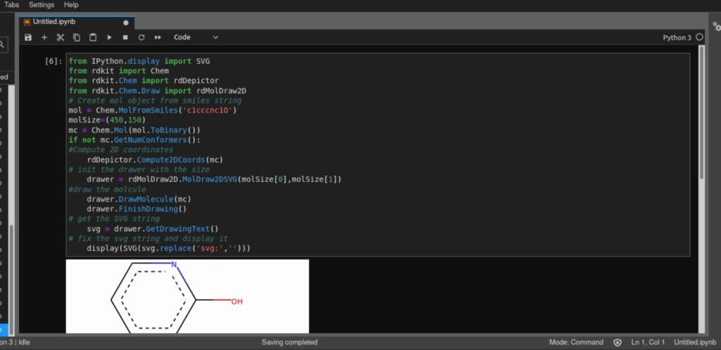
I was able to reproduce this sample for rdkit in a new python notebook:

1. Installed rdkit from Ubuntu's Software Manager on a VM hosted from Oracle's VirtualBox. 
2. Ran the sample Python code below and reproduced the output:

Sample code from  this site:  https://leedavies.dev/index.php/2018/10/06/rdkit-in-jupyter-notebooks/

This github also has samples:  
https://gist.github.com/vfscalfani/f10c4718e8d2e48586c48674a654aa20
https://github.com/rdkit/rdkit-tutorials
----------------

from IPython.display import SVG
from rdkit import Chem
from rdkit.Chem import rdDepictor
from rdkit.Chem.Draw import rdMolDraw2D
# Create mol object from smiles string
mol = Chem.MolFromSmiles('c1cccnc1O')
molSize=(450,150)
mc = Chem.Mol(mol.ToBinary())
if not mc.GetNumConformers():
#Compute 2D coordinates
    rdDepictor.Compute2DCoords(mc)
# init the drawer with the size
    drawer = rdMolDraw2D.MolDraw2DSVG(molSize[0],molSize[1])
#draw the molcule
    drawer.DrawMolecule(mc)
    drawer.FinishDrawing()
# get the SVG string
    svg = drawer.GetDrawingText()
# fix the svg string and display it
    display(SVG(svg.replace('svg:','')))

.
Status update. So far, so good. Even though it’s been well over a hundred calendar hours later, I haven’t made much progress since while loops. I’m currently in Lists. Now Lists is not the way I would normally go about programming, reason enough to pay more attention. I even downloaded another couple of free python texts for good measure.

Actually I’m almost completely engrossed in the news, including the apparently failed capitol coup and related events, it’s an ongoing crisis too big for me to ignore. I expect this historical ‘moment’ will not end till past the inauguration.

Sorry, slow python learning till then.
.

This company's free library is pretty good for visualizing. Like Nevyn's code it can take some time. http://docs.enthought.com/mayavi/mayavi/mlab.html#a-demo

To get you started, here is a pretty example showing a spherical harmonic as a surface:

# Create the data.
from numpy import pi, sin, cos, mgrid
dphi, dtheta = pi/250.0, pi/250.0
[phi,theta] = mgrid[0:pi+dphi*1.5:dphi,0:2*pi+dtheta*1.5:dtheta]
m0 = 4; m1 = 3; m2 = 2; m3 = 3; m4 = 6; m5 = 2; m6 = 6; m7 = 4;
r = sin(m0*phi)**m1 + cos(m2*phi)**m3 + sin(m4*theta)**m5 + cos(m6*theta)**m7
x = r*sin(phi)*cos(theta)
y = r*cos(phi)
z = r*sin(phi)*sin(theta)

# View it.
from mayavi import mlab
s = mlab.mesh(x, y, z)
mlab.show()
Bulk of the code in the above example is to create the data. One line suffices to visualize it. This produces the following visualization:

To get you started, here is a pretty example showing a spherical harmonic as a surface:

# Create the data.
from numpy import pi, sin, cos, mgrid
dphi, dtheta = pi/250.0, pi/250.0
[phi,theta] = mgrid[0:pi+dphi*1.5:dphi,0:2*pi+dtheta*1.5:dtheta]
m0 = 4; m1 = 3; m2 = 2; m3 = 3; m4 = 6; m5 = 2; m6 = 6; m7 = 4;
r = sin(m0*phi)**m1 + cos(m2*phi)**m3 + sin(m4*theta)**m5 + cos(m6*theta)**m7
x = r*sin(phi)*cos(theta)
y = r*cos(phi)
z = r*sin(phi)*sin(theta)

# View it.
from mayavi import mlab
s = mlab.mesh(x, y, z)
mlab.show()
Bulk of the code in the above example is to create the data. One line suffices to visualize it. This produces the following visualization:

.
That sure is a pretty spherical harmonic you got there Cr6. Definitely motivational. Then I see it gets better. According to SourceForge, download MayaVi at https://sourceforge.net/projects/mayavi/  

MayaVi is a free, cross platform, easy to use scientific data visualizer. It provides a GUI to ease the visualization process, is written in Python and uses the Visualization Toolkit (VTK) for the graphics.

I haven't downloaded MayaVi yet, any comments before I do? According to a document describing Mayavi by HAL, (Prabhu Ramachandran, Gaël Varoquaux) a multi-disciplinary open access library, over ten years ago,
https://core.ac.uk/download/pdf/208006248.pdf

VTK : The Visualization ToolKit [9] is one of the best, actively-developed, general-purpose, open-source, visualization and graphics libraries available.

Muy bueno Cr6. A free, high-class graphics application and library. That’s extremely motivating. No excuses now, must learn python. My progress there - I'm currently in the Dictionaries section.
.

Good question LTAM on the requirements. I have it installed on a 60 Gig Linux VM. It may have issues in a python notebook since it has an X windows gui.

This document has set up details.  https://docs.enthought.com/mayavi/mayavi/tips.html

This github page has details on installation as well and jupyter notebook support. https://github.com/larsoner/mayavi

Learning python can take a lot of time. I'm still working on it myself. Fortunately there are a lot of example .py scripts out there.

Finally have mlab-mavayi2 examples running on jupyter notebooks locally.  Here's a pretty cool example. 

Handles a lot like Nevyn's engine...LTAM, do you know if Nevyn's engine is still up and running somewhere on the web?



This is mlab.quiver3D can possibly render charge field flows?

Just ran this script in a new Jupyter notebook and it popped up the gui renderer for Mavayi:

----------

%gui qt

"""
An example showing the norm and phase of an atomic orbital: isosurfaces of
the norm, with colors  displaying the phase.
This example shows how you can apply a filter on one data set, and dislay
a second data set on the output of the filter. Here we use the contour
filter to extract isosurfaces of the norm of a complex field, and we
display the phase of the field with the colormap.
The field we choose to plot is a simplified version of the 3P_y atomic
orbital for hydrogen-like atoms.
The first step is to create a data source with two scalar datasets. The
second step is to apply filters and modules, using the
'set_active_attribute' filter to select on which data these apply.
Creating a data source with two scalar datasets is actually slightly
tricky, as it requires some understanding of the layout of the datasets
in TVTK. The reader is referred to :ref:`data-structures-used-by-mayavi`
for more details.
"""
# Author: Gael Varoquaux
# Copyright (c) 2008, Enthought, Inc.
# License: BSD Style.

# Create the data ############################################################
import numpy as np

x, y, z = np.ogrid[- .5:.5:200j, - .5:.5:200j, - .5:.5:200j]
r = np.sqrt(x ** 2 + y ** 2 + z ** 2)


# Generalized Laguerre polynomial (3, 2)
L = - r ** 3 / 6 + 5. / 2 * r ** 2 - 10 * r + 6

# Spherical harmonic (3, 2)
Y = (x + y * 1j) ** 2 * z / r ** 3

Phi = L * Y * np.exp(- r) * r ** 2

# Plot it ####################################################################
from mayavi import mlab
mlab.figure(1, fgcolor=(1, 1, 1), bgcolor=(0, 0, 0))
# We create a scalar field with the module of Phi as the scalar
src = mlab.pipeline.scalar_field(np.abs(Phi))

# And we add the phase of Phi as an additional array
# This is a tricky part: the layout of the new array needs to be the same
# as the existing dataset, and no checks are performed. The shape needs
# to be the same, and so should the data. Failure to do so can result in
# segfaults.
src.image_data.point_data.add_array(np.angle(Phi).T.ravel())
# We need to give a name to our new dataset.
src.image_data.point_data.get_array(1).name = 'angle'
# Make sure that the dataset is up to date with the different arrays:
src.update()

# We select the 'scalar' attribute, ie the norm of Phi
src2 = mlab.pipeline.set_active_attribute(src,
                                    point_scalars='scalar')

# Cut isosurfaces of the norm
contour = mlab.pipeline.contour(src2)

# Now we select the 'angle' attribute, ie the phase of Phi
contour2 = mlab.pipeline.set_active_attribute(contour,
                                    point_scalars='angle')

# And we display the surface. The colormap is the current attribute: the phase.
mlab.pipeline.surface(contour2, colormap='hsv')

mlab.colorbar(title='Phase', orientation='vertical', nb_labels=3)

mlab.show()

--------------------------------------

Here's a Lorenz equation example:
-------------

%gui qt

"""
An example displaying the trajectories for the Lorenz system of equations along with the z-nullcline.
The vector field of the Lorenz system flow is integrated to display trajectories using mlab's flow function:
:func:`mayavi.mlab.flow`.
The z-nullcline is plotted by extracting the z component of the vector field data source with the ExtractVectorComponent filter, and applying an IsoSurface module on this scalar component.
"""
# Author: Prabhu Ramachandran
# Copyright (c) 2008-2020, Enthought, Inc.
# License: BSD Style.

import numpy as np
from mayavi import mlab


def lorenz(x, y, z, s=10., r=28., b=8. / 3.):
    """The Lorenz system."""
    u = s * (y - x)
    v = r * x - y - x * z
    w = x * y - b * z
    return u, v, w

# Sample the space in an interesting region.
x, y, z = np.mgrid[-50:50:100j, -50:50:100j, -10:60:70j]
u, v, w = lorenz(x, y, z)
fig = mlab.figure(size=(400, 300), bgcolor=(0, 0, 0))

# Plot the flow of trajectories with suitable parameters.
f = mlab.flow(x, y, z, u, v, w, line_width=3, colormap='Paired')
f.module_manager.scalar_lut_manager.reverse_lut = True
f.stream_tracer.integration_direction = 'both'
f.stream_tracer.maximum_propagation = 200
# Uncomment the following line if you want to hide the seed:
#f.seed.widget.enabled = False

# Extract the z-velocity from the vectors and plot the 0 level set
# hence producing the z-nullcline.
src = f.mlab_source.m_data
e = mlab.pipeline.extract_vector_components(src)
e.component = 'z-component'
zc = mlab.pipeline.iso_surface(e, opacity=0.5, contours=[0, ],
            color=(0.6, 1, 0.2))
# When using transparency, hiding 'backface' triangles often gives better
# results
zc.actor.property.backface_culling = True

# A nice view of the plot.
mlab.view(140, 120, 113, [0.65, 1.5, 27])
mlab.show()

----------------




Magnetic Field Lines Example: 


"""
This example uses the streamline module to display field lines of a
magnetic dipole (a current loop).
This example requires scipy.
The magnetic field from an arbitrary current loop is calculated from
eqns (1) and (2) in Phys Rev A Vol. 35, N 4, pp. 1535-1546; 1987.
To get a prettier result, we use a fairly large grid to sample the
field. As a consequence, we need to clear temporary arrays as soon as
possible.
For a more thorough example of magnetic field calculation and
visualization with Mayavi and scipy, see
:ref:`example_magnetic_field`.
"""
# Author: Gael Varoquaux
# Copyright (c) 2007, Enthought, Inc.
# License: BSD Style.

import numpy as np
from scipy import special

#### Calculate the field ####################################################
radius = 1  # Radius of the coils

x, y, z = [e.astype(np.float32) for e in
            np.ogrid[-10:10:150j, -10:10:150j, -10:10:150j]]

# express the coordinates in polar form
rho = np.sqrt(x ** 2 + y ** 2)
x_proj = x / rho
y_proj = y / rho
# Free memory early
del x, y

E = special.ellipe((4 * radius * rho) / ((radius + rho) ** 2 + z ** 2))
K = special.ellipk((4 * radius * rho) / ((radius + rho) ** 2 + z ** 2))
Bz = 1 / np.sqrt((radius + rho) ** 2 + z ** 2) * (
                K
                + E * (radius ** 2 - rho ** 2 - z ** 2) /
                    ((radius - rho) ** 2 + z ** 2)
            )
Brho = z / (rho * np.sqrt((radius + rho) ** 2 + z ** 2)) * (
                - K
                + E * (radius ** 2 + rho ** 2 + z ** 2) /
                    ((radius - rho) ** 2 + z ** 2)
            )
del E, K, z, rho
# On the axis of the coil we get a divided by zero. This returns a
# NaN, where the field is actually zero :
Brho[np.isnan(Brho)] = 0

Bx, By = x_proj * Brho, y_proj * Brho

del x_proj, y_proj, Brho

#### Visualize the field ####################################################
from mayavi import mlab
fig = mlab.figure(1, size=(400, 400), bgcolor=(1, 1, 1), fgcolor=(0, 0, 0))

field = mlab.pipeline.vector_field(Bx, By, Bz)
# Unfortunately, the above call makes a copy of the arrays, so we delete
# this copy to free memory.
del Bx, By, Bz

magnitude = mlab.pipeline.extract_vector_norm(field)
contours = mlab.pipeline.iso_surface(magnitude,
                                        contours=[0.01, 0.8, 3.8, ],
                                        transparent=True,
                                        opacity=0.4,
                                        colormap='YlGnBu',
                                        vmin=0, vmax=2)


field_lines = mlab.pipeline.streamline(magnitude, seedtype='line',
                                        integration_direction='both',
                                        colormap='bone',
                                        vmin=0, vmax=1)

# Tweak a bit the streamline.
field_lines.stream_tracer.maximum_propagation = 100.
field_lines.seed.widget.point1 = [69, 75.5, 75.5]
field_lines.seed.widget.point2 = [82, 75.5, 75.5]
field_lines.seed.widget.resolution = 50
field_lines.seed.widget.enabled = False

mlab.view(42, 73, 104, [79,  75,  76])

mlab.show()

Here's the Chemistry.py example of H2O. Pretty basic rendering. Neyvn's engine looked better.

Location:  https://github.com/enthought/mayavi/tree/master/examples/mayavi/mlab

"""
In this example, we display the H2O molecule, and use volume rendering to display the electron localization function.
The atoms and the bounds are displayed using mlab.points3d and mlab.plot3d, with scalar information to control the color.
The electron localization function is displayed using volume rendering.
Good use of the `vmin` and `vmax` argument to `mlab.pipeline.volume` is critical to achieve a good visualization: the `vmin` threshold should placed high-enough for features to stand out.
The original is an electron localization function from Axel Kohlmeyer.
"""
# Author: Gael Varoquaux
# Copyright (c) 2008-2020, Enthought, Inc.
# License: BSD Style.

# Retrieve the electron localization data for H2O #############################

.
Cr6 wrote. Finally have mlab-mavayi2 examples running on jupyter notebooks locally. Here's a pretty cool example.
…
Airman. Sounds like eureka to me. Those are some fine examples. We can certainly “render charge field flows”, and then some. I’m sure you noticed the double toroid image for “norm and phase of an atomic orbital: isosurfaces of the norm, with colors displaying the phase” just needs a few tweaks in order to describe a charged particle’s photon/antiphoton emission field.

Thank you Sir, your examples make clear your idea to develop a python charge field library is definitely doable. Great, I see I have my work cut out for me.
 
Cr6 wrote. Do you know if Nevyn's engine is still up and running somewhere on the web?
Airman. Sorry, I don’t. Nor do I know what engine or engines he used to make his atomic models, I never tried using my browser console to peek at his code. I’m grateful he set up a few threejs projects in BitBucket, giving me the ‘permissions’ to make changes and learn from.
.

Re: AI Topics ...
https://milesmathis.forumotion.com/t617-ai-topics#6438
by Chromium6 Tuesday, 19 January at 12:53 am

I just hope we can get a few simple Juypter Notebooks on Miles' work, like Nevyn's C.F. Engine, that allows for further break-throughs. Obviously, when University researchers, CERN types, NASA types and lab experiments effectively show that as the time and space are reduce for measurements -- the "weirdness/unexpected" is not explainable especially at the nano-level. Hence Mathis or another revision of QT or something.  Like, Okay...you found these properties in matter.... now how do you explain it with accepted theory?  Miles' papers in a Notebook might point to some groundbreaking. Most published micro-bonding theory is pretty flimsly after new discoveries just basically invalidate their canon explanations with QT. Basically it is getting harder to match QT-80 year old theories with actual measurements/observations and I think some folks know it.

Airman. Made a copy of your AI Topics ... comment to the discussion here on the Miles' Periodic Table thread.

I agree. Sounds like a plan. I'm in.

Etc mentioned the wayback machine. I have no wayback application experience, maybe Nevyn's code is still viewable.
.

.

I finished reviewing the Python coding for non-programmers text, then watched a few Python and Jupyter videos. I decided to try downloading Anaconda, then downloading Jupyter from Anaconda. Everything seems to be up and running.

I'll see if I can open any of the example docs you posted above tomorrow.
.

.
Cr6 wrote. I just hope we can get a few simple Juypter Notebooks on Miles' work, like Nevyn's C.F. Engine, that allows for further break-throughs. …

Airman. Agreed.

There are no doubt many decisions necessary; currently, all I have are questions. Since this was your idea and you have notebook experience, please consider yourself in charge. In other words, I'll be the happy worker bee, and you make the command decisions.

For starters, what is our first jupyter notebook charge field topic? If I may suggest, given this thread, and the fact Nevyn’s Lab and all his work is gone*, how about we build a charge field model Periodic Table? Let the user select and view the individual elements.

Meanwhile, I’m still learning. I haven’t figured out how to access Mayavi yet. I don't see any separate application; is it built-into the anaconda install, am I supposed to import it into an individual notebook with an 'import ipy' command?

P.S. Update, status wise. My current immediate difficulty/question is - how do I go about opening up .ipynb files from the web? Don't worry, I'm not asking you yet. I see Jupyter allows one to select a file source location. Keep at it.

* Drat and double drat, I don’t think I could program anything as well as Nevyn.
.

Okay LTAM,

I'm on the hook for this. I just need to remember about interesting stuff I looked at 6 months ago. Will try a spin up some good notebooks. Try to get Jupyter running on Spark as well. It can allow for a good database to be added.

.


Good, but don't look too fast, I forgot it all. I have a new machine, so I downloaded the latest (free) individual user Anaconda version. Jupyter is up and running. I'll go through the Anaconda-cloud Getting Started with Anaconda Literacy and Fertility example case to get refamiliarized and properly launched ...
.

.
The fertility/literacy anaconda-cloud example quickly broke down trying to download the requested wiki data – 404 error – although I did download the two applicable data files from Gapminder.org.

I carried on by reviewing a few anaconda and jupyter tutorials and writing a few new notebook files including using matplotlib to create various plots and graphs.  

http://docs.enthought.com/mayavi/mayavi/index.html
http://docs.enthought.com/mayavi/mayavi/mlab.html#simple-scripting-with-mlab
I believe what originally interested you in suggesting some jupyter notebook project in the first place was learning about Mayavi, and seeing its excellent scientific/mathematical diagrams. Mayavi is the only anaconda compatible program (after a couple of searches) that might allow us to animate - rotate 3D shapes. While not initially installed (200+ modules) by anaconda, the mayavi module is available for download (one of hundreds of thousands of modules) at any time if desired.  

I haven’t downloaded it yet because the documentation includes explicit directions (shown below) about Using it with Ipython and Matplotlib that I haven’t made sense of yet. Are these downloading instructions or instructions for each and every code block importing instance?
 
If you want to use Matplotlib’s interactive plotting with Mayavi’s mlab in IPython you should:
start IPython with:
$ ipython --matplotlib=qt
alternatively, start IPython with the –gui=qt option:
$ ipython --gui=qt
and before importing any matplotlib modules, enter the following Python commands:
>>> import matplotlib
>>> matplotlib.use('Qt4Agg')
>>> matplotlib.interactive(True)
one could also use the --pylab option to IPython as follows:
$ ipython --pylab=qt
If you want matplotlib and mlab to work together by default in IPython, you can change you default matplotlib backend, by editing the ~/.matplotlib/matplotlibrc to add the following line:
...

I spent some time looking at the anaconda installed Spyder, a much nicer coding environment than notepad++. Anaconda can also install R, but I’d need to create a “new environment” in order to do so.

I looked at Adobe Sparks. https://www.youtube.com/watch?v=3zH5LNt8dH8

How to Use Adobe Spark - Beginner's Tutorial. I appreciate the ease of designing a website by adding/modifying images, text, videos and audio. https://www.adobe.com/express/pricing I see 3 choices: 1. a “free starter plan” where one may “pick from thousands of free images and icons for your designs”; 2. an individual plan, free for 30 days and $10/month thereafter; and 3. the team plan is $20/month. I didn’t download it, I wouldn’t spend money on it unless you had a good reason, such as actually designing a website.

Sorry I was side tracked by pi9 and some other topics Cr6. I suppose I should try re-reading this thread from the start, any directions you provide would be received with complete attention and be greatly appreciated.
.

.

I think I’m good to go Cr6. Mayavi is up and running with Jupyter notebook – creating its own active screen plots with adjustable size and viewpoints. After an initial conflict between python 3.8 and mayavi, I created and switched to new environment using python 3.7 which is compatible. The image shows a parabaloid created by matplotlib and rotated by mayavi mlab. The initial parabaloid code and discussion can be found in a Stack Overflow question, how to rotate a 3D surface in matplotlib. https://stackoverflow.com/questions/38326983/how-to-rotate-a-3d-surface-in-matplotlib

I also properly completed the initial female literacy versus birthrate example and a few others. It’s very nice following along and creating live outputs.
.

Awesome LTAM... maybe we can get a library up and running with Nevyn's old code? Would be real cool if we could.

https://github.com/jupyter-widgets/pythreejs

.
A Library is an awesome vision Cr6. For the time being I’m just trying to provide positive progress reports. For example, I enjoyed typing along (with plenty of pausing and repeated plays) all the examples in a good 3hr video, 3D Visualization with Mayavi | SciPy 2018 Tutorial | Prabhu Ramachandran. https://www.youtube.com/watch?v=r6OD07Qq2mw

I have a few quibbles, such as: What were the questions? But then I didn’t download any of the available source files. I’ll need to review it again in the future. I’d definitely recommend it to others.

And what a surprise, pythreejs! I must admit, despite my serious trepidations, anaconda3 (or the anaconda navigator) has made what would have been very difficult or impossible installs in the past – Prabhu mentioned mayavi is among the worst - rather easy. Pythreejs is now installed on my machine and available to my jupyter notebook. I’m in the middle of reviewing the documentation, and retyping the exercises at, https://pythreejs.readthedocs.io/en/stable/examples/index.html


The above image is recreated from the examples animation section.
 
pythreejs mimics threejs, but there are several significant differences. I don’t know how Nevyn programmed his atomic models, but I do know threejs, at least well enough that I shouldn’t have much difficulty in building atoms. All that’s needed are two different sized spheres (electrons and neutrons), and disc-like elipsoids (protons), properly oriented and positioned. If you think I should ask for Nevyn’s help, I will; otherwise I'll attempt to do so without it. Feel free to task or advise me as you see fit.

How about if I try starting with a relatively easy (I hope) notebook project, such as recreating jfmeyer’s phi-based origin? All that’s needed are: a grid, axes, points, lines, squares, rectangles, circles, labels; maybe later allow some interaction to verify labeled values. Unfortunately I don’t believe pythreejs, mayavi, or matplotlib can make accurate, interactive geometric diagrams or plots. jfmeyers uses desmos but I don’t see that listed as an available python package. Turtle graphics is too clunky. Do you know any good python geometric diagramming programs? Maybe some canvas based program?
.

.

The above shows the output of my first jupyter notebook program, recreating a phi-based origin using ipycanvas. I believe ipycanvas is limited in that it can only draw images and does not support 3d plotting; still, the code includes all the x and y points shown, and might be transferred to a real plotting program. At the other end of the spectrum there’s an autocad version of python that requires the user to work with autocad documents. I’m hoping there’s a jupyter compatible program or two available somewhere between the two. I’ll cross post the image and code on jfmeyer’s phi-based origin thread.

Code:


# Draw a phi-based origin

from ipycanvas import Canvas
from math import pi, sqrt

# The plot is square, with extra margin on the right for dimensions.
isquare = 400  # scaling plot to the desired canvas size
center = isquare/2
half = isquare/10 # sized slightly greater than 1+sqrt(5)/2
unit = isquare/5 # the scalar between 1 and the canvas sq's side length
pradius = 0.02*unit  # used for dimensional points
bradius = (sqrt(5)/2)*unit # r=sqrt(5)/2  circle
cradius = (1/2)*(sqrt(5)+2)*unit # r=(sqrt(5)/2)+1  circle

pwidth = isquare+1.6*unit
canvas = Canvas(width=pwidth, height=isquare)

# Grid s = 4.6, with lines every 0.1
canvas.stroke_style = 'gray'
#canvas.set_line_dash  # not used
grid = 4.6
i = 0
while i <= grid:
        canvas.stroke_line(center + (i - grid/2)*unit, center-grid/2*unit, center + (i - 2.3)*unit, center+grid/2*unit)
        canvas.stroke_line(center - grid/2*unit, center-(i - grid/2)*unit, center + grid/2*unit, center-(i - grid/2)*unit)
        i += 0.1

# Clear the grid from the unit square area
canvas.fill_style = 'white'
canvas.fill_rect(center - half, center - half, unit, unit)   

# r=1/2 circle
canvas.fill_style = 'yellow'
canvas.fill_circle(center, center, half)

# Axes
canvas.stroke_style = 'green'
canvas.stroke_line(center-cradius, center, center+cradius, center)
canvas.stroke_line(center, center-cradius, center, center+cradius)

# Remove the yellow from the r=1/2 circle from within the s=1/sqrt(2) square
canvas.fill_style = 'white'
canvas.begin_path()
canvas.move_to(center, center + half)
canvas.line_to(center + half, center)
canvas.line_to(center, center - half)
canvas.line_to(center - half, center)
canvas.fill()

# Unit square
canvas.stroke_style = 'red'
canvas.move_to(center, center + half)
canvas.stroke_line(center - half, center + half, center + half, center + half)
canvas.stroke_line(center + half, center + half, center + half, center - half)
canvas.stroke_line(center + half, center - half, center - half, center - half)
canvas.stroke_line(center - half, center - half, center - half, center + half)
#canvas.stroke_rects(center, center, 2*unit, unit)
# The Last line is no good. The stroke_rects command kept bombing - exceeding the
# Jupyter tab memory. No rectangles - must draw each line separately.

# Draw r=1/2, r=sqrt(5)/2 and r=(sqrt(5)/2)+1 circles
canvas.stroke_style = 'blue'
canvas.stroke_circle(center, center, half) # r=1/2 circle
canvas.stroke_style = 'black'
canvas.stroke_circle(center, center, bradius)  # r=sqrt(5)/2  circle
canvas.stroke_circle(center, center, cradius)  # r=(sqrt(5)/2)+1  circle

# 1/sqrt(0.5) square, D1, D2, D3, D4
canvas.stroke_style = 'black'
canvas.stroke_line(center, center - half, center + half, center)
canvas.stroke_line(center + half, center, center, center + half)
canvas.stroke_line(center, center + half, center - half, center)
canvas.stroke_line(center - half, center, center, center - half)

# Horiz 2x1 rectangles (left and right halves) with sqrt(5) diagonals
canvas.stroke_style = 'black'
canvas.stroke_line(center - half, center - half, center - unit, center - half)
canvas.stroke_line(center - unit, center - half, center - unit, center + half)
canvas.stroke_line(center - unit, center + half, center - half, center + half)
canvas.stroke_line(center + half, center - half, center + unit, center - half)
canvas.stroke_line(center + unit, center - half, center + unit, center + half)
canvas.stroke_line(center + unit, center + half, center + half, center + half)
canvas.stroke_line(center - unit, center - half, center + unit, center + half)
canvas.stroke_line(center - unit, center + half, center + unit, center - half)

# Vert 2x1 rectangles (Top and bottom halves) with sqrt(5) diagonals
canvas.stroke_line(center - half, center - half, center - half, center - unit)
canvas.stroke_line(center - half, center - unit, center + half, center - unit)
canvas.stroke_line(center + half, center - unit, center + half, center - half)
canvas.stroke_line(center - half, center + half, center - half, center + unit)
canvas.stroke_line(center - half, center + unit, center + half, center + unit)
canvas.stroke_line(center + half, center + unit, center + half, center + half)
canvas.stroke_line(center - half, center - unit, center + half, center + unit)
canvas.stroke_line(center - half, center + unit, center + half, center - unit)

# Dimension lines and points
#canvas.fill_style = 'black'
canvas.font = '15px serif'
canvas.stroke_style = 'red'
canvas.fill_style = 'red'
canvas.stroke_line(center, center - cradius, center + cradius + 1.2*unit, center - cradius)
canvas.stroke_line(center, center + cradius, center + cradius + 1.2*unit, center + cradius)
canvas.stroke_line(center + cradius + 1.2*unit, center - cradius, center + cradius + 1.2*unit, center + cradius)
canvas.fill_circle(center + cradius + 1.2*unit, center - cradius, pradius) # point
canvas.stroke_circle(center + cradius + 1.2*unit, center + cradius, pradius) # point

canvas.stroke_line(center + cradius + 0.4*unit, center - bradius, center + cradius + 0.4*unit, center - cradius)
canvas.stroke_circle(center + cradius + 0.4*unit, center - bradius, pradius)
canvas.stroke_circle(center + cradius + 0.4*unit, center - cradius, pradius)

canvas.stroke_line(center + unit, center - half, center + cradius + 0.4*unit, center - half)
canvas.stroke_line(center + cradius + 0.4*unit, center - half, center + cradius + 0.4*unit, center + half)
canvas.stroke_line(center + cradius + 0.4*unit, center + half, center + unit, center + half)
canvas.stroke_circle(center + cradius + 0.4*unit, center - half, pradius)
canvas.stroke_circle(center + cradius + 0.4*unit, center + half, pradius)

canvas.stroke_line(center + cradius + 0.4*unit, center + bradius, center + cradius + 0.4*unit, center + cradius)
canvas.stroke_circle(center + cradius + 0.4*unit, center + bradius, pradius)
canvas.stroke_circle(center + cradius + 0.4*unit, center + cradius, pradius)

canvas.stroke_line(center, center - bradius, center + cradius + 0.6*unit, center - bradius)
canvas.stroke_line(center, center + bradius, center + cradius + 0.6*unit, center + bradius)
canvas.stroke_line(center + cradius + 0.6*unit, center - bradius, center + cradius + 0.6*unit, center + bradius)
canvas.stroke_circle(center + cradius + 0.6*unit, center - bradius, pradius)
canvas.stroke_circle(center + cradius + 0.6*unit, center + bradius, pradius)

canvas.stroke_line(center, center - half, center + cradius + 0.8*unit, center - half)
canvas.stroke_line(center + cradius + 0.8*unit, center - half, center + cradius + 0.8*unit, center - cradius)
canvas.stroke_circle(center + cradius + 0.8*unit, center - half, pradius)
canvas.stroke_circle(center + cradius + 0.8*unit, center - cradius, pradius)

canvas.stroke_line(center, center + half, center + cradius + unit, center + half)
canvas.stroke_line(center + cradius + unit, center + half, center + cradius + unit, center - cradius)
canvas.stroke_circle(center + cradius + unit, center - cradius, pradius)
canvas.stroke_circle(center + cradius + unit, center + half, pradius)

# Dimension text. First remove the red dimension lines where the dimension text will be placed.
# The different colors helped, so I left them in.
#canvas.fill_style = 'black'
#canvas.fill_style = 'red'
canvas.fill_style = 'white'
tlocx = center + cradius + 0.4*unit - 0.15*unit
tlocy = center - cradius + bradius/2 - 0.2*unit
canvas.fill_rect(tlocx, tlocy, 0.3*unit, 0.3*unit)
canvas.fill_style = 'black'
tlocxb = center + cradius + 0.37*unit # + 0.01*unit
tlocyb = center - cradius + bradius/2 + 0.015*unit
canvas.fill_text('1', tlocxb, tlocyb)

#canvas.fill_style = 'cyan'
canvas.fill_style = 'white'
tlocx = center + cradius + 0.4*unit - 0.15*unit
tlocy = center - 0.15*unit
canvas.fill_rect(tlocx, tlocy, 0.3*unit, 0.3*unit)
canvas.fill_style = 'black'
tlocxb = center + cradius + 0.37*unit # + 0.01*unit
tlocyb = center + 0.07*unit # 0.15*unit
canvas.fill_text('1', tlocxb, tlocyb)

#canvas.fill_style = 'yellow'
canvas.fill_style = 'white'
tlocx = center + cradius + 0.4*unit - 0.15*unit
tlocy = center + cradius - bradius/2 - 0.1*unit
canvas.fill_rect(tlocx, tlocy, 0.3*unit, 0.3*unit)
canvas.fill_style = 'black'
tlocxb = center + cradius + 0.37*unit
tlocyb = center + cradius - bradius/2 + 0.115*unit
canvas.fill_text('1', tlocxb, tlocyb)

#canvas.fill_style = 'magenta'
canvas.fill_style = 'white'
tlocx = center + cradius + 0.6*unit - 0.15*unit
tlocy = center - 0.15*unit
canvas.fill_rect(tlocx, tlocy, 0.3*unit, 0.3*unit)
canvas.fill_style = 'black'
tlocxb = center + cradius + 0.2*unit + 0.3*unit
tlocyb = tlocyb = center + 0.07*unit
canvas.fill_text('√5', tlocxb, tlocyb)

#canvas.fill_style = 'green'
canvas.fill_style = 'white'
tlocx = center + cradius + 0.8*unit - 0.15*unit
tlocy = center - cradius + (cradius - half)/2 - 0.15*unit
canvas.fill_rect(tlocx, tlocy, 0.8*unit, 0.3*unit)
canvas.fill_style = 'black'
tlocxb = center + cradius + 0.8*unit - 0.12*unit
tlocyb = center - cradius + (cradius - half)/2 + 0.06*unit
canvas.fill_text('Φ^1=Φ^2-1', tlocxb, tlocyb)

#canvas.fill_style = 'orange'
canvas.fill_style = 'white'
tlocx = center + cradius + unit - 0.15*unit
tlocy = center + half - cradius + (cradius - half)/2 - 0.15*unit 
canvas.fill_rect(tlocx, tlocy, 1.5*unit, 0.3*unit)
canvas.fill_style = 'black'
tlocxb = center + cradius + unit - 0.1*unit
tlocyb = center + half - cradius + (cradius - half)/2 + 0.06*unit
canvas.fill_text('Φ^2=Φ+1', tlocxb, tlocyb)

canvas.fill_style = 'white'
tlocx = center + cradius + 1.2*unit - 0.15*unit
tlocy = center - 0.15*unit
canvas.fill_rect(tlocx, tlocy, 0.3*unit, 0.3*unit)
canvas.fill_style = 'black'
#tlocxb = center + cradius + 1.1*unit
tlocxb = center + cradius + 1.075*unit
tlocyb = tlocyb = center + 0.07*unit
canvas.fill_text('Φ^3=√5+2', tlocxb, tlocyb)

# Image border
canvas.stroke_style = 'black'
canvas.stroke_line(0, 0,pwidth, 0)
canvas.stroke_line(pwidth, 0, pwidth, isquare)
canvas.stroke_line(pwidth, isquare, 0, isquare)
canvas.stroke_line(0, isquare, 0, 0)

canvas


P.S. Made several changes to clean up the code - no change to the image.
.

.

Another phi-based origin diagram.

This image shows my second jupyter notebook effort at creating a phi-based origin. This time using pythreejs. I say again, pythreejs is not a 3D plotting program, it is an objects based language where lines are usually edges, more suited to positioning 3D spheres in space than plotting accurate diagrams. For example, CircleGeometry approximates circles with polygons, two dimensional polygonal disc meshes, not open circles, one must indicate or default to the circle’s number of sides.

As far as I know, all pythreejs curves must be broken into line segments. Separate subject, in threejs and windows, lines thicker than a single pixel is a problem. And sorry, there’s no title. I haven’t figured out how to import text, and I don’t believe I will. I thought about it before, and used it in an earlier project. I recall, Nevyn obliged me by making it available but mentioned it would be better to avoid text unless it was absolutely necessary. Maybe pythreejs code can be ported into a mayavi graph?

The code I wrote to create the output shown began as the Read the Docs, pythreejs code example, Thick Line Geometry.
https://pythreejs.readthedocs.io/en/stable/examples/ThickLines.html

Utilizing LineSegmentGeometry we do have thick lines and interesting coloring possibilities. The mouse’s pythreejs orbital camera control can swivel the image about. Also each plotted component: grid, axes, halfSq, halfrCir, unitSq, keplerRL, keplerTB, s5d2rCir, and s5p2d2rCir can be switched on and off – live -using the blue checkboxes at the bottom, an ipywidget. I cropped the other 6 checkboxes extended to the right, rather than modifying the image by adding them as extra rows at the bottom, or capturing the entire screen image.

I was unable to get any array building push commands to work. The solution I came up with was in generating so-called LineSegmentGeometry ‘positions’ arrays, the x, y, z endpoints, from and to, for each of the diagram’s line segments. A bit cumbersome to say the least, like ensuring that last array character, a comma, is omitted. And the LineSegments ‘positions’ array is (may or may not be) followed by a ‘colors’ array of the same length. On the other hand it works. I used 40 line segments for each of the circles shown in the image, but reduced that number to 12 in order to shorten the printed code’s length (40:12) - but results in an uglier output.

For the ipycanvas code last time, I copy/pasted the text of a single jupyter netbook code block ( In[]: ). This time there are 15 code blocks. I opened the file with notebook++ ipynb format, and will post it as such. At 974 lines I may need to break it into sections.

Cr6, If you can find the time and would be so kind, please let me know if you can get it to run under jupyter notebook. Or perhaps suggest some other alternative.

PhyOrg.ipynb

Code:


{
 "cells": [
  {
   "cell_type": "code",
   "execution_count": 103,
   "id": "035e1a0e",
   "metadata": {},
   "outputs": [],
   "source": [
    "# Creating a phi-based origin diagram. Adapted from the pythreejs example, Thick Line \n",
    "# Geometry at https://pythreejs.readthedocs.io/en/stable/examples/ThickLines.html\n",
    "\n",
    "from pythreejs import *\n",
    "from IPython.display import display\n",
    "from ipywidgets import VBox, HBox, Checkbox, jslink\n",
    "from math import pi, sqrt, atan, sin, cos\n",
    "import numpy as np"
   ]
  },
  {
   "cell_type": "code",
   "execution_count": 104,
   "id": "92929fe0",
   "metadata": {},
   "outputs": [],
   "source": [
    "# Camera, lights.\n",
    "\n",
    "view_width = 500\n",
    "view_height = 400\n",
    "center = 0\n",
    "unit = 1\n",
    "half = 0.5\n",
    "#pradius = 0.02*unit  # used for dimensional points - not yet used\n",
    "bradius = (sqrt(5)/2)*unit # r=sqrt(5)/2  circle\n",
    "cradius = (1/2)*(sqrt(5)+2)*unit # r=(sqrt(5)/2)+1  circle\n",
    "\n",
    "camera = PerspectiveCamera(45, position=[0, 0, 5], aspect=view_width/view_height)  # Star\n",
    " \n",
    "key_light = DirectionalLight(position=[0, 10, 0])\n",
    "ambient_light = AmbientLight()"
   ]
  },
  {
   "cell_type": "code",
   "execution_count": 105,
   "id": "295ec7ac",
   "metadata": {},
   "outputs": [
    {
     "name": "stdout",
     "output_type": "stream",
     "text": [
      "[[ 0.43301270189221935 , 0.24999999999999997 , 0], [ 0.25000000000000006 ,  0.4330127018922193 , 0]],\n",
      "[[ 0.25000000000000006 , 0.4330127018922193 , 0], [ 3.061616997868383e-17 ,  0.5 , 0]],\n",
      "[[ 3.061616997868383e-17 , 0.5 , 0], [ -0.2499999999999999 ,  0.43301270189221935 , 0]],\n",
      "[[ -0.2499999999999999 , 0.43301270189221935 , 0], [ -0.43301270189221935 ,  0.24999999999999997 , 0]],\n",
      "[[ -0.43301270189221935 , 0.24999999999999997 , 0], [ -0.5 ,  6.123233995736766e-17 , 0]],\n",
      "[[ -0.5 , 6.123233995736766e-17 , 0], [ -0.4330127018922193 ,  -0.25000000000000006 , 0]],\n",
      "[[ -0.4330127018922193 , -0.25000000000000006 , 0], [ -0.2500000000000002 ,  -0.43301270189221924 , 0]],\n",
      "[[ -0.2500000000000002 , -0.43301270189221924 , 0], [ -9.184850993605148e-17 ,  -0.5 , 0]],\n",
      "[[ -9.184850993605148e-17 , -0.5 , 0], [ 0.25000000000000006 ,  -0.4330127018922193 , 0]],\n",
      "[[ 0.25000000000000006 , -0.4330127018922193 , 0], [ 0.4330127018922192 ,  -0.2500000000000002 , 0]],\n",
      "[[ 0.4330127018922192 , -0.2500000000000002 , 0], [ 0.5 ,  -1.2246467991473532e-16 , 0]],\n",
      "[[ 0.5 , -1.2246467991473532e-16 , 0], [ 0.43301270189221935 ,  0.24999999999999997 , 0]]\n"
     ]
    }
   ],
   "source": [
    "# Circle, LineSegmentsGeometry position array generator. In order to use \n",
    "# LineSegmentsGeometry, one must approximate the circle as some high number \n",
    "# of \"segments\"- sided polygon. Specifying the radius and number of segments, \n",
    "# this block will output each line segment endpoint x,y,z, coords 'positions'  \n",
    "# array. Copy/paste the array into the object's LineSegmentGeometry et voila. \n",
    "\n",
    "radius = 1/2;          # The output 1s used for the r=1/2 circle.\n",
    "# radius = sqrt(5)/2;    # The output is used for the sqrt(5)/2 circle.\n",
    "# radius = (sqrt(5)+2)/2;  # The output is used for the (sqrt(5)+2)/2 circle.\n",
    "# segments = 40;         # Used for the posted image,  \n",
    "segments = 12;           # Shorter code but uglier circles. \n",
    "theta_next = 0;\n",
    "x_next = 0;\n",
    "y_next = 0; \n",
    "j = 0;\n",
    "i = 0;\n",
    "\n",
    "while i <= (segments - 1):\n",
    "    theta = ((i + 1) / segments) * pi * 2.0;\n",
    "    x = radius * cos(theta);\n",
    "    y = radius * sin(theta);\n",
    "    j = i + 2;\n",
    "    if( (j - 1) == segments ): j = 1;\n",
    "    theta_next = (j / segments) * pi * 2.0;\n",
    "    x_next = radius * cos(theta_next);\n",
    "    y_next = radius * sin(theta_next);\n",
    "    if i == segments - 1:\n",
    "        print('[[', x,',', y,', 0], [', x_next,', ', y_next,', 0]]')\n",
    "    else:\n",
    "        print('[[', x,',', y,', 0], [', x_next,', ', y_next,', 0]],')\n",
    "    i += 1  "
   ]
  },
  {
   "cell_type": "code",
   "execution_count": 122,
   "id": "14940b6f",
   "metadata": {},
   "outputs": [
    {
     "name": "stdout",
     "output_type": "stream",
     "text": [
      "[[ -2.3 , -2.3 , 0 ], [ -2.3 ,  2.3 ,  0 ]],\n",
      "[[ -2.3 , -2.3 , 0 ], [ 2.3 ,  -2.3 ,  0 ]],\n",
      "[[ -2.2 , -2.3 , 0 ], [ -2.2 ,  2.3 ,  0 ]],\n",
      "[[ -2.3 , -2.2 , 0 ], [ 2.3 ,  -2.2 ,  0 ]],\n",
      "[[ -2.1 , -2.3 , 0 ], [ -2.1 ,  2.3 ,  0 ]],\n",
      "[[ -2.3 , -2.1 , 0 ], [ 2.3 ,  -2.1 ,  0 ]],\n",
      "[[ -2.0 , -2.3 , 0 ], [ -2.0 ,  2.3 ,  0 ]],\n",
      "[[ -2.3 , -2.0 , 0 ], [ 2.3 ,  -2.0 ,  0 ]],\n",
      "[[ -1.9 , -2.3 , 0 ], [ -1.9 ,  2.3 ,  0 ]],\n",
      "[[ -2.3 , -1.9 , 0 ], [ 2.3 ,  -1.9 ,  0 ]],\n",
      "[[ -1.8 , -2.3 , 0 ], [ -1.8 ,  2.3 ,  0 ]],\n",
      "[[ -2.3 , -1.8 , 0 ], [ 2.3 ,  -1.8 ,  0 ]],\n",
      "[[ -1.7 , -2.3 , 0 ], [ -1.7 ,  2.3 ,  0 ]],\n",
      "[[ -2.3 , -1.7 , 0 ], [ 2.3 ,  -1.7 ,  0 ]],\n",
      "[[ -1.6 , -2.3 , 0 ], [ -1.6 ,  2.3 ,  0 ]],\n",
      "[[ -2.3 , -1.6 , 0 ], [ 2.3 ,  -1.6 ,  0 ]],\n",
      "[[ -1.5 , -2.3 , 0 ], [ -1.5 ,  2.3 ,  0 ]],\n",
      "[[ -2.3 , -1.5 , 0 ], [ 2.3 ,  -1.5 ,  0 ]],\n",
      "[[ -1.4 , -2.3 , 0 ], [ -1.4 ,  2.3 ,  0 ]],\n",
      "[[ -2.3 , -1.4 , 0 ], [ 2.3 ,  -1.4 ,  0 ]],\n",
      "[[ -1.3 , -2.3 , 0 ], [ -1.3 ,  2.3 ,  0 ]],\n",
      "[[ -2.3 , -1.3 , 0 ], [ 2.3 ,  -1.3 ,  0 ]],\n",
      "[[ -1.2 , -2.3 , 0 ], [ -1.2 ,  2.3 ,  0 ]],\n",
      "[[ -2.3 , -1.2 , 0 ], [ 2.3 ,  -1.2 ,  0 ]],\n",
      "[[ -1.1 , -2.3 , 0 ], [ -1.1 ,  2.3 ,  0 ]],\n",
      "[[ -2.3 , -1.1 , 0 ], [ 2.3 ,  -1.1 ,  0 ]],\n",
      "[[ -1.0 , -2.3 , 0 ], [ -1.0 ,  2.3 ,  0 ]],\n",
      "[[ -2.3 , -1.0 , 0 ], [ 2.3 ,  -1.0 ,  0 ]],\n",
      "[[ -0.9 , -2.3 , 0 ], [ -0.9 ,  2.3 ,  0 ]],\n",
      "[[ -2.3 , -0.9 , 0 ], [ 2.3 ,  -0.9 ,  0 ]],\n",
      "[[ -0.8 , -2.3 , 0 ], [ -0.8 ,  2.3 ,  0 ]],\n",
      "[[ -2.3 , -0.8 , 0 ], [ 2.3 ,  -0.8 ,  0 ]],\n",
      "[[ -0.7 , -2.3 , 0 ], [ -0.7 ,  2.3 ,  0 ]],\n",
      "[[ -2.3 , -0.7 , 0 ], [ 2.3 ,  -0.7 ,  0 ]],\n",
      "[[ -0.6 , -2.3 , 0 ], [ -0.6 ,  2.3 ,  0 ]],\n",
      "[[ -2.3 , -0.6 , 0 ], [ 2.3 ,  -0.6 ,  0 ]],\n",
      "[[ -0.5 , -2.3 , 0 ], [ -0.5 ,  2.3 ,  0 ]],\n",
      "[[ -2.3 , -0.5 , 0 ], [ 2.3 ,  -0.5 ,  0 ]],\n",
      "[[ -0.4 , -2.3 , 0 ], [ -0.4 ,  2.3 ,  0 ]],\n",
      "[[ -2.3 , -0.4 , 0 ], [ 2.3 ,  -0.4 ,  0 ]],\n",
      "[[ -0.3 , -2.3 , 0 ], [ -0.3 ,  2.3 ,  0 ]],\n",
      "[[ -2.3 , -0.3 , 0 ], [ 2.3 ,  -0.3 ,  0 ]],\n",
      "[[ -0.2 , -2.3 , 0 ], [ -0.2 ,  2.3 ,  0 ]],\n",
      "[[ -2.3 , -0.2 , 0 ], [ 2.3 ,  -0.2 ,  0 ]],\n",
      "[[ -0.1 , -2.3 , 0 ], [ -0.1 ,  2.3 ,  0 ]],\n",
      "[[ -2.3 , -0.1 , 0 ], [ 2.3 ,  -0.1 ,  0 ]],\n",
      "[[ 0.0 , -2.3 , 0 ], [ 0.0 ,  2.3 ,  0 ]],\n",
      "[[ -2.3 , 0.0 , 0 ], [ 2.3 ,  0.0 ,  0 ]],\n",
      "[[ 0.1 , -2.3 , 0 ], [ 0.1 ,  2.3 ,  0 ]],\n",
      "[[ -2.3 , 0.1 , 0 ], [ 2.3 ,  0.1 ,  0 ]],\n",
      "[[ 0.2 , -2.3 , 0 ], [ 0.2 ,  2.3 ,  0 ]],\n",
      "[[ -2.3 , 0.2 , 0 ], [ 2.3 ,  0.2 ,  0 ]],\n",
      "[[ 0.3 , -2.3 , 0 ], [ 0.3 ,  2.3 ,  0 ]],\n",
      "[[ -2.3 , 0.3 , 0 ], [ 2.3 ,  0.3 ,  0 ]],\n",
      "[[ 0.4 , -2.3 , 0 ], [ 0.4 ,  2.3 ,  0 ]],\n",
      "[[ -2.3 , 0.4 , 0 ], [ 2.3 ,  0.4 ,  0 ]],\n",
      "[[ 0.5 , -2.3 , 0 ], [ 0.5 ,  2.3 ,  0 ]],\n",
      "[[ -2.3 , 0.5 , 0 ], [ 2.3 ,  0.5 ,  0 ]],\n",
      "[[ 0.6 , -2.3 , 0 ], [ 0.6 ,  2.3 ,  0 ]],\n",
      "[[ -2.3 , 0.6 , 0 ], [ 2.3 ,  0.6 ,  0 ]],\n",
      "[[ 0.7 , -2.3 , 0 ], [ 0.7 ,  2.3 ,  0 ]],\n",
      "[[ -2.3 , 0.7 , 0 ], [ 2.3 ,  0.7 ,  0 ]],\n",
      "[[ 0.8 , -2.3 , 0 ], [ 0.8 ,  2.3 ,  0 ]],\n",
      "[[ -2.3 , 0.8 , 0 ], [ 2.3 ,  0.8 ,  0 ]],\n",
      "[[ 0.9 , -2.3 , 0 ], [ 0.9 ,  2.3 ,  0 ]],\n",
      "[[ -2.3 , 0.9 , 0 ], [ 2.3 ,  0.9 ,  0 ]],\n",
      "[[ 1.0 , -2.3 , 0 ], [ 1.0 ,  2.3 ,  0 ]],\n",
      "[[ -2.3 , 1.0 , 0 ], [ 2.3 ,  1.0 ,  0 ]],\n",
      "[[ 1.1 , -2.3 , 0 ], [ 1.1 ,  2.3 ,  0 ]],\n",
      "[[ -2.3 , 1.1 , 0 ], [ 2.3 ,  1.1 ,  0 ]],\n",
      "[[ 1.2 , -2.3 , 0 ], [ 1.2 ,  2.3 ,  0 ]],\n",
      "[[ -2.3 , 1.2 , 0 ], [ 2.3 ,  1.2 ,  0 ]],\n",
      "[[ 1.3 , -2.3 , 0 ], [ 1.3 ,  2.3 ,  0 ]],\n",
      "[[ -2.3 , 1.3 , 0 ], [ 2.3 ,  1.3 ,  0 ]],\n",
      "[[ 1.4 , -2.3 , 0 ], [ 1.4 ,  2.3 ,  0 ]],\n",
      "[[ -2.3 , 1.4 , 0 ], [ 2.3 ,  1.4 ,  0 ]],\n",
      "[[ 1.5 , -2.3 , 0 ], [ 1.5 ,  2.3 ,  0 ]],\n",
      "[[ -2.3 , 1.5 , 0 ], [ 2.3 ,  1.5 ,  0 ]],\n",
      "[[ 1.6 , -2.3 , 0 ], [ 1.6 ,  2.3 ,  0 ]],\n",
      "[[ -2.3 , 1.6 , 0 ], [ 2.3 ,  1.6 ,  0 ]],\n",
      "[[ 1.7 , -2.3 , 0 ], [ 1.7 ,  2.3 ,  0 ]],\n",
      "[[ -2.3 , 1.7 , 0 ], [ 2.3 ,  1.7 ,  0 ]],\n",
      "[[ 1.8 , -2.3 , 0 ], [ 1.8 ,  2.3 ,  0 ]],\n",
      "[[ -2.3 , 1.8 , 0 ], [ 2.3 ,  1.8 ,  0 ]],\n",
      "[[ 1.9 , -2.3 , 0 ], [ 1.9 ,  2.3 ,  0 ]],\n",
      "[[ -2.3 , 1.9 , 0 ], [ 2.3 ,  1.9 ,  0 ]],\n",
      "[[ 2.0 , -2.3 , 0 ], [ 2.0 ,  2.3 ,  0 ]],\n",
      "[[ -2.3 , 2.0 , 0 ], [ 2.3 ,  2.0 ,  0 ]],\n",



The first 200 lines.
.

.
lines 201 to 600.

Code:


      "[[ 2.1 , -2.3 , 0 ], [ 2.1 ,  2.3 ,  0 ]],\n",
      "[[ -2.3 , 2.1 , 0 ], [ 2.3 ,  2.1 ,  0 ]],\n",
      "[[ 2.2 , -2.3 , 0 ], [ 2.2 ,  2.3 ,  0 ]],\n",
      "[[ -2.3 , 2.2 , 0 ], [ 2.3 ,  2.2 ,  0 ]],\n",
      "[[ 2.3 , -2.3 , 0 ], [ 2.3 ,  2.3 ,  0 ]],\n",
      "[[ -2.3 , 2.3 , 0 ], [ 2.3 ,  2.3 ,  0 ]],\n"
     ]
    }
   ],
   "source": [
    "# Grid, LineSegmentsGeometry grid endpoints position array generator. The\n",
    "# output position array will be be used to create a grid in the next block.\n",
    "# changed 0.1 to 0.2 to shorten the code\n",
    "\n",
    "x=0\n",
    "y=0\n",
    "z=0\n",
    "i = 0\n",
    "while i <= 4.6:\n",
    "    xv = round(center+(i - 2.3)*unit,1)\n",
    "    yv = round(center-2.3*unit,1)   \n",
    "    zv = 0\n",
    "    xv_next = round(center+(i - 2.3)*unit,1)\n",
    "    yv_next = round(center+2.3*unit,1)\n",
    "    zv_next = 0 \n",
    "    xh = round(center-2.3*unit,1)     \n",
    "    yh = round(center+(i - 2.3)*unit,1) \n",
    "    zh = 0\n",
    "    xh_next = round(center+2.3*unit,1) \n",
    "    yh_next = round(center+(i - 2.3)*unit,1) \n",
    "    zh_next = 0\n",
    "    print('[[', xv,',', yv,',', zv,'], [', xv_next,', ', yv_next,', ', zv_next,']],')\n",
    "    print('[[', xh,',', yh,',', zh,'], [', xh_next,', ', yh_next,', ', zh_next,']],')\n",
    "    i += 0.1    \n"
   ]
  },
  {
   "cell_type": "code",
   "execution_count": 123,
   "id": "61616970",
   "metadata": {},
   "outputs": [
    {
     "data": {
      "application/vnd.jupyter.widget-view+json": {
       "model_id": "1b8cb71b50b145c7b5c59fcb7d789585",
       "version_major": 2,
       "version_minor": 0
      },
      "text/plain": [
       "Preview(child=LineSegments2(geometry=LineSegmentsGeometry(colors=array([[[0., 1., 0.],\n",
       "        [0., 1., 0.]],\n",
       "…"
      ]
     },
     "metadata": {},
     "output_type": "display_data"
    }
   ],
   "source": [
    "# Grid.  s=4.6. 46 each X and Y lines, every 0.1. \n",
    "\n",
    "gridG = LineSegmentsGeometry(\n",
    "    positions=[\n",
    "[[ -2.3 , -2.3 , 0 ], [ -2.3 ,  2.3 ,  0 ]],\n",
    "[[ -2.3 , -2.3 , 0 ], [ 2.3 ,  -2.3 ,  0 ]],\n",
    "[[ -2.2 , -2.3 , 0 ], [ -2.2 ,  2.3 ,  0 ]],\n",
    "[[ -2.3 , -2.2 , 0 ], [ 2.3 ,  -2.2 ,  0 ]],\n",
    "[[ -2.1 , -2.3 , 0 ], [ -2.1 ,  2.3 ,  0 ]],\n",
    "[[ -2.3 , -2.1 , 0 ], [ 2.3 ,  -2.1 ,  0 ]],\n",
    "[[ -2.0 , -2.3 , 0 ], [ -2.0 ,  2.3 ,  0 ]],\n",
    "[[ -2.3 , -2.0 , 0 ], [ 2.3 ,  -2.0 ,  0 ]],\n",
    "[[ -1.9 , -2.3 , 0 ], [ -1.9 ,  2.3 ,  0 ]],\n",
    "[[ -2.3 , -1.9 , 0 ], [ 2.3 ,  -1.9 ,  0 ]],\n",
    "[[ -1.8 , -2.3 , 0 ], [ -1.8 ,  2.3 ,  0 ]],\n",
    "[[ -2.3 , -1.8 , 0 ], [ 2.3 ,  -1.8 ,  0 ]],\n",
    "[[ -1.7 , -2.3 , 0 ], [ -1.7 ,  2.3 ,  0 ]],\n",
    "[[ -2.3 , -1.7 , 0 ], [ 2.3 ,  -1.7 ,  0 ]],\n",
    "[[ -1.6 , -2.3 , 0 ], [ -1.6 ,  2.3 ,  0 ]],\n",
    "[[ -2.3 , -1.6 , 0 ], [ 2.3 ,  -1.6 ,  0 ]],\n",
    "[[ -1.5 , -2.3 , 0 ], [ -1.5 ,  2.3 ,  0 ]],\n",
    "[[ -2.3 , -1.5 , 0 ], [ 2.3 ,  -1.5 ,  0 ]],\n",
    "[[ -1.4 , -2.3 , 0 ], [ -1.4 ,  2.3 ,  0 ]],\n",
    "[[ -2.3 , -1.4 , 0 ], [ 2.3 ,  -1.4 ,  0 ]],\n",
    "[[ -1.3 , -2.3 , 0 ], [ -1.3 ,  2.3 ,  0 ]],\n",
    "[[ -2.3 , -1.3 , 0 ], [ 2.3 ,  -1.3 ,  0 ]],\n",
    "[[ -1.2 , -2.3 , 0 ], [ -1.2 ,  2.3 ,  0 ]],\n",
    "[[ -2.3 , -1.2 , 0 ], [ 2.3 ,  -1.2 ,  0 ]],\n",
    "[[ -1.1 , -2.3 , 0 ], [ -1.1 ,  2.3 ,  0 ]],\n",
    "[[ -2.3 , -1.1 , 0 ], [ 2.3 ,  -1.1 ,  0 ]],\n",
    "[[ -1.0 , -2.3 , 0 ], [ -1.0 ,  2.3 ,  0 ]],\n",
    "[[ -2.3 , -1.0 , 0 ], [ 2.3 ,  -1.0 ,  0 ]],\n",
    "[[ -0.9 , -2.3 , 0 ], [ -0.9 ,  2.3 ,  0 ]],\n",
    "[[ -2.3 , -0.9 , 0 ], [ 2.3 ,  -0.9 ,  0 ]],\n",
    "[[ -0.8 , -2.3 , 0 ], [ -0.8 ,  2.3 ,  0 ]],\n",
    "[[ -2.3 , -0.8 , 0 ], [ 2.3 ,  -0.8 ,  0 ]],\n",
    "[[ -0.7 , -2.3 , 0 ], [ -0.7 ,  2.3 ,  0 ]],\n",
    "[[ -2.3 , -0.7 , 0 ], [ 2.3 ,  -0.7 ,  0 ]],\n",
    "[[ -0.6 , -2.3 , 0 ], [ -0.6 ,  2.3 ,  0 ]],\n",
    "[[ -2.3 , -0.6 , 0 ], [ 2.3 ,  -0.6 ,  0 ]],\n",
    "[[ -0.5 , -2.3 , 0 ], [ -0.5 ,  2.3 ,  0 ]],\n",
    "[[ -2.3 , -0.5 , 0 ], [ 2.3 ,  -0.5 ,  0 ]],\n",
    "[[ -0.4 , -2.3 , 0 ], [ -0.4 ,  2.3 ,  0 ]],\n",
    "[[ -2.3 , -0.4 , 0 ], [ 2.3 ,  -0.4 ,  0 ]],\n",
    "[[ -0.3 , -2.3 , 0 ], [ -0.3 ,  2.3 ,  0 ]],\n",
    "[[ -2.3 , -0.3 , 0 ], [ 2.3 ,  -0.3 ,  0 ]],\n",
    "[[ -0.2 , -2.3 , 0 ], [ -0.2 ,  2.3 ,  0 ]],\n",
    "[[ -2.3 , -0.2 , 0 ], [ 2.3 ,  -0.2 ,  0 ]],\n",
    "[[ -0.1 , -2.3 , 0 ], [ -0.1 ,  2.3 ,  0 ]],\n",
    "[[ -2.3 , -0.1 , 0 ], [ 2.3 ,  -0.1 ,  0 ]],\n",
    "[[ 0.0 , -2.3 , 0 ], [ 0.0 ,  2.3 ,  0 ]],\n",
    "[[ -2.3 , 0.0 , 0 ], [ 2.3 ,  0.0 ,  0 ]],\n",
    "[[ 0.1 , -2.3 , 0 ], [ 0.1 ,  2.3 ,  0 ]],\n",
    "[[ -2.3 , 0.1 , 0 ], [ 2.3 ,  0.1 ,  0 ]],\n",
    "[[ 0.2 , -2.3 , 0 ], [ 0.2 ,  2.3 ,  0 ]],\n",
    "[[ -2.3 , 0.2 , 0 ], [ 2.3 ,  0.2 ,  0 ]],\n",
    "[[ 0.3 , -2.3 , 0 ], [ 0.3 ,  2.3 ,  0 ]],\n",
    "[[ -2.3 , 0.3 , 0 ], [ 2.3 ,  0.3 ,  0 ]],\n",
    "[[ 0.4 , -2.3 , 0 ], [ 0.4 ,  2.3 ,  0 ]],\n",
    "[[ -2.3 , 0.4 , 0 ], [ 2.3 ,  0.4 ,  0 ]],\n",
    "[[ 0.5 , -2.3 , 0 ], [ 0.5 ,  2.3 ,  0 ]],\n",
    "[[ -2.3 , 0.5 , 0 ], [ 2.3 ,  0.5 ,  0 ]],\n",
    "[[ 0.6 , -2.3 , 0 ], [ 0.6 ,  2.3 ,  0 ]],\n",
    "[[ -2.3 , 0.6 , 0 ], [ 2.3 ,  0.6 ,  0 ]],\n",
    "[[ 0.7 , -2.3 , 0 ], [ 0.7 ,  2.3 ,  0 ]],\n",
    "[[ -2.3 , 0.7 , 0 ], [ 2.3 ,  0.7 ,  0 ]],\n",
    "[[ 0.8 , -2.3 , 0 ], [ 0.8 ,  2.3 ,  0 ]],\n",
    "[[ -2.3 , 0.8 , 0 ], [ 2.3 ,  0.8 ,  0 ]],\n",
    "[[ 0.9 , -2.3 , 0 ], [ 0.9 ,  2.3 ,  0 ]],\n",
    "[[ -2.3 , 0.9 , 0 ], [ 2.3 ,  0.9 ,  0 ]],\n",
    "[[ 1.0 , -2.3 , 0 ], [ 1.0 ,  2.3 ,  0 ]],\n",
    "[[ -2.3 , 1.0 , 0 ], [ 2.3 ,  1.0 ,  0 ]],\n",
    "[[ 1.1 , -2.3 , 0 ], [ 1.1 ,  2.3 ,  0 ]],\n",
    "[[ -2.3 , 1.1 , 0 ], [ 2.3 ,  1.1 ,  0 ]],\n",
    "[[ 1.2 , -2.3 , 0 ], [ 1.2 ,  2.3 ,  0 ]],\n",
    "[[ -2.3 , 1.2 , 0 ], [ 2.3 ,  1.2 ,  0 ]],\n",
    "[[ 1.3 , -2.3 , 0 ], [ 1.3 ,  2.3 ,  0 ]],\n",
    "[[ -2.3 , 1.3 , 0 ], [ 2.3 ,  1.3 ,  0 ]],\n",
    "[[ 1.4 , -2.3 , 0 ], [ 1.4 ,  2.3 ,  0 ]],\n",
    "[[ -2.3 , 1.4 , 0 ], [ 2.3 ,  1.4 ,  0 ]],\n",
    "[[ 1.5 , -2.3 , 0 ], [ 1.5 ,  2.3 ,  0 ]],\n",
    "[[ -2.3 , 1.5 , 0 ], [ 2.3 ,  1.5 ,  0 ]],\n",
    "[[ 1.6 , -2.3 , 0 ], [ 1.6 ,  2.3 ,  0 ]],\n",
    "[[ -2.3 , 1.6 , 0 ], [ 2.3 ,  1.6 ,  0 ]],\n",
    "[[ 1.7 , -2.3 , 0 ], [ 1.7 ,  2.3 ,  0 ]],\n",
    "[[ -2.3 , 1.7 , 0 ], [ 2.3 ,  1.7 ,  0 ]],\n",
    "[[ 1.8 , -2.3 , 0 ], [ 1.8 ,  2.3 ,  0 ]],\n",
    "[[ -2.3 , 1.8 , 0 ], [ 2.3 ,  1.8 ,  0 ]],\n",
    "[[ 1.9 , -2.3 , 0 ], [ 1.9 ,  2.3 ,  0 ]],\n",
    "[[ -2.3 , 1.9 , 0 ], [ 2.3 ,  1.9 ,  0 ]],\n",
    "[[ 2.0 , -2.3 , 0 ], [ 2.0 ,  2.3 ,  0 ]],\n",
    "[[ -2.3 , 2.0 , 0 ], [ 2.3 ,  2.0 ,  0 ]],\n",
    "[[ 2.1 , -2.3 , 0 ], [ 2.1 ,  2.3 ,  0 ]],\n",
    "[[ -2.3 , 2.1 , 0 ], [ 2.3 ,  2.1 ,  0 ]],\n",
    "[[ 2.2 , -2.3 , 0 ], [ 2.2 ,  2.3 ,  0 ]],\n",
    "[[ -2.3 , 2.2 , 0 ], [ 2.3 ,  2.2 ,  0 ]],\n",
    "[[ 2.3 , -2.3 , 0 ], [ 2.3 ,  2.3 ,  0 ]],\n",
    "[[ -2.3 , 2.3 , 0 ], [ 2.3 ,  2.3 ,  0 ]]\n",
    "        ],\n",
    "        colors=[\n",
    "            [[0, 1, 0], [0, 1, 0]],\n",
    "            [[0, 1, 0], [0, 1, 0]],\n",
    "            [[0, 1, 0], [0, 1, 0]],\n",
    "            [[0, 1, 0], [0, 1, 0]],\n",
    "            [[0, 1, 0], [0, 1, 0]],\n",
    "            [[0, 1, 0], [0, 1, 0]],\n",
    "            [[0, 1, 0], [0, 1, 0]],\n",
    "            [[0, 1, 0], [0, 1, 0]],\n",
    "            [[0, 1, 0], [0, 1, 0]],\n",
    "            [[0, 1, 0], [0, 1, 0]],\n",
    "            [[0, 1, 0], [0, 1, 0]],\n",
    "            [[0, 1, 0], [0, 1, 0]],\n",
    "            [[0, 1, 0], [0, 1, 0]],\n",
    "            [[0, 1, 0], [0, 1, 0]],\n",
    "            [[0, 1, 0], [0, 1, 0]],\n",
    "            [[0, 1, 0], [0, 1, 0]],\n",
    "            [[0, 1, 0], [0, 1, 0]],\n",
    "            [[0, 1, 0], [0, 1, 0]],\n",
    "            [[0, 1, 0], [0, 1, 0]],\n",
    "            [[0, 1, 0], [0, 1, 0]],\n",
    "            [[0, 1, 0], [0, 1, 0]],\n",
    "            [[0, 1, 0], [0, 1, 0]],\n",
    "            [[0, 1, 0], [0, 1, 0]],\n",
    "            [[0, 1, 0], [0, 1, 0]],\n",
    "            [[0, 1, 0], [0, 1, 0]],\n",
    "            [[0, 1, 0], [0, 1, 0]],\n",
    "            [[0, 1, 0], [0, 1, 0]],\n",
    "            [[0, 1, 0], [0, 1, 0]],\n",
    "            [[0, 1, 0], [0, 1, 0]],\n",
    "            [[0, 1, 0], [0, 1, 0]],\n",
    "            [[0, 1, 0], [0, 1, 0]],\n",
    "            [[0, 1, 0], [0, 1, 0]],\n",
    "            [[0, 1, 0], [0, 1, 0]],\n",
    "            [[0, 1, 0], [0, 1, 0]],\n",
    "            [[0, 1, 0], [0, 1, 0]],\n",
    "            [[0, 1, 0], [0, 1, 0]],\n",
    "            [[0, 1, 0], [0, 1, 0]],\n",
    "            [[0, 1, 0], [0, 1, 0]],\n",
    "            [[0, 1, 0], [0, 1, 0]],\n",
    "            [[0, 1, 0], [0, 1, 0]],\n",
    "            [[0, 1, 0], [0, 1, 0]],\n",
    "            [[0, 1, 0], [0, 1, 0]],\n",
    "            [[0, 1, 0], [0, 1, 0]],\n",
    "            [[0, 1, 0], [0, 1, 0]],\n",
    "            [[0, 1, 0], [0, 1, 0]],\n",
    "            [[0, 1, 0], [0, 1, 0]],\n",
    "            [[0, 1, 0], [0, 1, 0]],\n",
    "            [[0, 1, 0], [0, 1, 0]],\n",
    "            [[0, 1, 0], [0, 1, 0]],\n",
    "            [[0, 1, 0], [0, 1, 0]],\n",
    "            [[0, 1, 0], [0, 1, 0]],\n",
    "            [[0, 1, 0], [0, 1, 0]],\n",
    "            [[0, 1, 0], [0, 1, 0]],\n",
    "            [[0, 1, 0], [0, 1, 0]],\n",
    "            [[0, 1, 0], [0, 1, 0]],\n",
    "            [[0, 1, 0], [0, 1, 0]],\n",
    "            [[0, 1, 0], [0, 1, 0]],\n",
    "            [[0, 1, 0], [0, 1, 0]],\n",
    "            [[0, 1, 0], [0, 1, 0]],\n",
    "            [[0, 1, 0], [0, 1, 0]],\n",
    "            [[0, 1, 0], [0, 1, 0]],\n",
    "            [[0, 1, 0], [0, 1, 0]],\n",
    "            [[0, 1, 0], [0, 1, 0]],\n",
    "            [[0, 1, 0], [0, 1, 0]],\n",
    "            [[0, 1, 0], [0, 1, 0]],\n",
    "            [[0, 1, 0], [0, 1, 0]],\n",
    "            [[0, 1, 0], [0, 1, 0]],\n",
    "            [[0, 1, 0], [0, 1, 0]],\n",
    "            [[0, 1, 0], [0, 1, 0]],\n",
    "            [[0, 1, 0], [0, 1, 0]],\n",
    "            [[0, 1, 0], [0, 1, 0]],\n",
    "            [[0, 1, 0], [0, 1, 0]],\n",
    "            [[0, 1, 0], [0, 1, 0]],\n",
    "            [[0, 1, 0], [0, 1, 0]],\n",
    "            [[0, 1, 0], [0, 1, 0]],\n",
    "            [[0, 1, 0], [0, 1, 0]],\n",
    "            [[0, 1, 0], [0, 1, 0]],\n",
    "            [[0, 1, 0], [0, 1, 0]],\n",
    "            [[0, 1, 0], [0, 1, 0]],\n",
    "            [[0, 1, 0], [0, 1, 0]],\n",
    "            [[0, 1, 0], [0, 1, 0]],\n",
    "            [[0, 1, 0], [0, 1, 0]],\n",
    "            [[0, 1, 0], [0, 1, 0]],\n",
    "            [[0, 1, 0], [0, 1, 0]],\n",
    "            [[0, 1, 0], [0, 1, 0]],\n",
    "            [[0, 1, 0], [0, 1, 0]],\n",
    "            [[0, 1, 0], [0, 1, 0]],\n",
    "            [[0, 1, 0], [0, 1, 0]],\n",
    "            [[0, 1, 0], [0, 1, 0]],\n",
    "            [[0, 1, 0], [0, 1, 0]],\n",
    "            [[0, 1, 0], [0, 1, 0]],\n",
    "            [[0, 1, 0], [0, 1, 0]],\n",
    "            [[0, 1, 0], [0, 1, 0]],\n",
    "            [[0, 1, 0], [0, 1, 0]]\n",
    "    ],    \n",
    ")\n",
    "gridM = LineMaterial(linewidth=1, vertexColors='VertexColors')\n",
    "grid = LineSegments2(gridG, gridM)\n",
    "grid"
   ]
  },
  {
   "cell_type": "code",
   "execution_count": 124,
   "id": "88dd6945",
   "metadata": {},
   "outputs": [
    {
     "data": {
      "application/vnd.jupyter.widget-view+json": {
       "model_id": "95e07747dfd0420aa238bc2636037fe5",
       "version_major": 2,
       "version_minor": 0
      },
      "text/plain": [
       "Preview(child=LineSegments2(geometry=LineSegmentsGeometry(positions=array([[[-2.118034,  0.      ,  0.      ],…"
      ]
     },
     "metadata": {},
     "output_type": "display_data"
    }
   ],
   "source": [
    "# Axes. Not included in output diagram, showing the LineSegmentGeometry \n",
    "# colors array is replaced with a single color.\n",
    "\n",
    "axesG = LineSegmentsGeometry(\n",
    "    positions=[\n",
    "            [[center-cradius, center, 0], [center+cradius, center, 0]],\n",
    "            [[center, center-cradius, 0], [center, center+cradius, 0]]\n",
    "        ],\n",
    ")\n",
    "axesM = LineMaterial(linewidth=2, color='gray')\n",
    "axes = LineSegments2(axesG, axesM)\n",
    "axes\n"
   ]
  },
  {
   "cell_type": "code",
   "execution_count": 125,
   "id": "5c6f42e0",
   "metadata": {},
   "outputs": [
    {
     "data": {
      "application/vnd.jupyter.widget-view+json": {
       "model_id": "235f4d13e73144acb26fc6c5235dcc6c",
       "version_major": 2,
       "version_minor": 0
      },
      "text/plain": [
       "Preview(child=LineSegments2(geometry=LineSegmentsGeometry(colors=array([[[0., 1., 1.],\n",
       "        [0., 1., 1.]],\n",
       "…"
      ]
     },
     "metadata": {},
     "output_type": "display_data"
    }
   ],
   "source": [
    "# S=1/2 square.\n",
    "\n",
    "halfS = LineSegmentsGeometry(\n",
    "    positions=[\n",
    "            [[center, center + half, 0], [center + half, center, 0]],\n",
    "            [[center + half, center, 0], [center, center - half, 0]],\n",
    "            [[center, center - half, 0], [center - half, center, 0]],\n",
    "            [[center - half, center, 0], [center, center + half, 0]]\n",
    "        ],\n",
    "        colors=[\n",
    "            [[0, 1, 1], [0, 1, 1]],\n",
    "            [[0, 1, 1], [0, 1, 1]],\n",
    "            [[0, 1, 1], [0, 1, 1]],\n",
    "            [[0, 1, 1], [0, 1, 1]]\n",
    "    ],    \n",
    ")\n",
    "halfM = LineMaterial(linewidth=3, vertexColors='VertexColors')\n",
    "halfSq = LineSegments2(halfS, halfM)\n",
    "halfSq\n",
    "#print(halfS)\n",
    "\n"
   ]
  },
  {
   "cell_type": "code",
   "execution_count": 126,
   "id": "945cd680",
   "metadata": {},
   "outputs": [
    {
     "data": {
      "application/vnd.jupyter.widget-view+json": {
       "model_id": "d0d1c9989b3b488a95b7fe319a7377ee",
       "version_major": 2,
       "version_minor": 0
      },
      "text/plain": [
       "Preview(child=LineSegments2(geometry=LineSegmentsGeometry(colors=array([[[0., 0., 1.],\n",
       "        [0., 0., 1.]],\n",
       "…"
      ]
     },
     "metadata": {},
     "output_type": "display_data"
    }
   ],
   "source": [
    "# r=1/2 circle\n",
    "halfCG = LineSegmentsGeometry(\n",
    "    positions=[\n",
    "[[ 0.43301270189221935 , 0.24999999999999997 , 0], [ 0.25000000000000006 ,  0.4330127018922193 , 0]],\n",
    "[[ 0.25000000000000006 , 0.4330127018922193 , 0], [ 3.061616997868383e-17 ,  0.5 , 0]],\n",
    "[[ 3.061616997868383e-17 , 0.5 , 0], [ -0.2499999999999999 ,  0.43301270189221935 , 0]],\n",
    "[[ -0.2499999999999999 , 0.43301270189221935 , 0], [ -0.43301270189221935 ,  0.24999999999999997 , 0]],\n",
    "[[ -0.43301270189221935 , 0.24999999999999997 , 0], [ -0.5 ,  6.123233995736766e-17 , 0]],\n",
    "[[ -0.5 , 6.123233995736766e-17 , 0], [ -0.4330127018922193 ,  -0.25000000000000006 , 0]],\n",
    "[[ -0.4330127018922193 , -0.25000000000000006 , 0], [ -0.2500000000000002 ,  -0.43301270189221924 , 0]],\n",
    "[[ -0.2500000000000002 , -0.43301270189221924 , 0], [ -9.184850993605148e-17 ,  -0.5 , 0]],\n",
    "[[ -9.184850993605148e-17 , -0.5 , 0], [ 0.25000000000000006 ,  -0.4330127018922193 , 0]],\n",
    "[[ 0.25000000000000006 , -0.4330127018922193 , 0], [ 0.4330127018922192 ,  -0.2500000000000002 , 0]],\n",
    "[[ 0.4330127018922192 , -0.2500000000000002 , 0], [ 0.5 ,  -1.2246467991473532e-16 , 0]],\n",
    "[[ 0.5 , -1.2246467991473532e-16 , 0], [ 0.43301270189221935 ,  0.24999999999999997 , 0]]\n",
    "    ],\n",
    "    colors=[\n",
    "        [[0, 0, 1], [0, 0, 1]],\n",
    "        [[0, 0, 1], [0, 0, 1]],\n",
    "        [[0, 0, 1], [0, 0, 1]],\n",
    "        [[0, 0, 1], [0, 0, 1]],\n",
    "        [[0, 0, 1], [0, 0, 1]],\n",
    "        [[0, 0, 1], [0, 0, 1]],\n",
    "        [[0, 0, 1], [0, 0, 1]],\n",
    "        [[0, 0, 1], [0, 0, 1]],\n",
    "        [[0, 0, 1], [0, 0, 1]],\n",
    "        [[0, 0, 1], [0, 0, 1]],\n",
    "        [[0, 0, 1], [0, 0, 1]],\n",
    "        [[0, 0, 1], [0, 0, 1]],\n",
    "        [[0, 0, 1], [0, 0, 1]]\n",
    "    ],\n",
    ")\n",


.
lines 601-974

Code:


    "halfCM = LineMaterial(linewidth=3, vertexColors='VertexColors')\n",
    "halfrCir = LineSegments2(halfCG, halfCM)\n",
    "halfrCir\n"
   ]
  },
  {
   "cell_type": "code",
   "execution_count": 127,
   "id": "27283419",
   "metadata": {},
   "outputs": [
    {
     "data": {
      "application/vnd.jupyter.widget-view+json": {
       "model_id": "a5859109c9c847cca25e6d3596880537",
       "version_major": 2,
       "version_minor": 0
      },
      "text/plain": [
       "Preview(child=LineSegments2(geometry=LineSegmentsGeometry(colors=array([[[1., 0., 0.],\n",
       "        [1., 0., 0.]],\n",
       "…"
      ]
     },
     "metadata": {},
     "output_type": "display_data"
    }
   ],
   "source": [
    "unitS = LineSegmentsGeometry(\n",
    "    positions=[\n",
    "            [[center - half, center - half, 0], [center + half, center - half, 0]],\n",
    "            [[center + half, center - half, 0], [center + half, center + half, 0]],\n",
    "            [[center + half, center + half, 0], [center - half, center + half, 0]],\n",
    "            [[center - half, center + half, 0], [center - half, center - half, 0]]\n",
    "        ],\n",
    "        colors=[\n",
    "            [[1, 0, 0], [1, 0, 0]],\n",
    "            [[1, 0, 0], [1, 0, 0]],\n",
    "            [[1, 0, 0], [1, 0, 0]],\n",
    "            [[1, 0, 0], [1, 0, 0]]\n",
    "    ],    \n",
    ")\n",
    "unitM = LineMaterial(linewidth=3, vertexColors='VertexColors')\n",
    "unitSq = LineSegments2(unitS, unitM)\n",
    "unitSq"
   ]
  },
  {
   "cell_type": "code",
   "execution_count": 128,
   "id": "bac8e6e0",
   "metadata": {},
   "outputs": [
    {
     "data": {
      "application/vnd.jupyter.widget-view+json": {
       "model_id": "62c54c673b0a4398b7af256f5ba6d82f",
       "version_major": 2,
       "version_minor": 0
      },
      "text/plain": [
       "Preview(child=LineSegments2(geometry=LineSegmentsGeometry(colors=array([[[1., 0., 1.],\n",
       "        [1., 0., 1.]],\n",
       "…"
      ]
     },
     "metadata": {},
     "output_type": "display_data"
    }
   ],
   "source": [
    "# Horiz 2x1 rectangles with sqrt(5) diagonals\n",
    "keplerrlG = LineSegmentsGeometry(\n",
    "    positions=[\n",
    "            [[center - half, center - half, 0], [center - unit, center - half, 0]],\n",
    "            [[center - unit, center - half, 0], [center - unit, center + half, 0]],\n",
    "            [[center - unit, center + half, 0], [center - half, center + half, 0]],\n",
    "            [[center + half, center - half, 0], [center + unit, center - half, 0]],\n",
    "            [[center + unit, center - half, 0], [center + unit, center + half, 0]],\n",
    "            [[center + unit, center + half, 0], [center + half, center + half, 0]],\n",
    "            [[center - unit, center - half, 0], [center + unit, center + half, 0]],\n",
    "            [[center - unit, center + half, 0], [center + unit, center - half, 0]]           \n",
    "        ],\n",
    "        colors=[\n",
    "            [[1, 0, 1], [1, 0, 1]],\n",
    "            [[1, 0, 1], [1, 0, 1]],\n",
    "            [[1, 0, 1], [1, 0, 1]],\n",
    "            [[1, 0, 1], [1, 0, 1]],\n",
    "            [[1, 0, 1], [1, 0, 1]],\n",
    "            [[1, 0, 1], [1, 0, 1]],\n",
    "            [[1, 0, 1], [1, 0, 1]],\n",
    "            [[1, 0, 1], [1, 0, 1]]\n",
    "    ],    \n",
    ")\n",
    "keplerrlM = LineMaterial(linewidth=1, vertexColors='VertexColors')\n",
    "keplerRL = LineSegments2(keplerrlG, keplerrlM)\n",
    "keplerRL"
   ]
  },
  {
   "cell_type": "code",
   "execution_count": 129,
   "id": "b153352d",
   "metadata": {},
   "outputs": [
    {
     "data": {
      "application/vnd.jupyter.widget-view+json": {
       "model_id": "2236ad4c2bc440b88bc92440335ca9f1",
       "version_major": 2,
       "version_minor": 0
      },
      "text/plain": [
       "Preview(child=LineSegments2(geometry=LineSegmentsGeometry(colors=array([[[1., 0., 1.],\n",
       "        [1., 0., 1.]],\n",
       "…"
      ]
     },
     "metadata": {},
     "output_type": "display_data"
    }
   ],
   "source": [
    "# Vert 2x1 rectangles with sqrt(5) diagonals\n",
    "keplertbG = LineSegmentsGeometry(\n",
    "    positions=[\n",
    "            [[center - half, center - half, 0], [center - half, center - unit, 0]],\n",
    "            [[center - half, center - unit, 0], [center + half, center - unit, 0]],\n",
    "            [[center + half, center - unit, 0], [center + half, center - half, 0]],\n",
    "            [[center - half, center + half, 0], [center - half, center + unit, 0]],\n",
    "            [[center - half, center + unit, 0], [center + half, center + unit, 0]],\n",
    "            [[center + half, center + unit, 0], [center + half, center + half, 0]],\n",
    "            [[center - half, center - unit, 0], [center + half, center + unit, 0]],\n",
    "            [[center - half, center + unit, 0], [center + half, center - unit, 0]]           \n",
    "        ],\n",
    "        colors=[\n",
    "            [[1, 0, 1], [1, 0, 1]],\n",
    "            [[1, 0, 1], [1, 0, 1]],\n",
    "            [[1, 0, 1], [1, 0, 1]],\n",
    "            [[1, 0, 1], [1, 0, 1]],\n",
    "            [[1, 0, 1], [1, 0, 1]],\n",
    "            [[1, 0, 1], [1, 0, 1]],\n",
    "            [[1, 0, 1], [1, 0, 1]],\n",
    "            [[1, 0, 1], [1, 0, 1]]\n",
    "    ],    \n",
    ")\n",
    "keplertbM = LineMaterial(linewidth=1, vertexColors='VertexColors')\n",
    "keplerTB = LineSegments2(keplertbG, keplertbM)\n",
    "keplerTB"
   ]
  },
  {
   "cell_type": "code",
   "execution_count": 130,
   "id": "bc67775c",
   "metadata": {},
   "outputs": [
    {
     "data": {
      "application/vnd.jupyter.widget-view+json": {
       "model_id": "cb885b06d9f54771b9569e684fa9c900",
       "version_major": 2,
       "version_minor": 0
      },
      "text/plain": [
       "Preview(child=LineSegments2(geometry=LineSegmentsGeometry(colors=array([[[0., 0., 1.],\n",
       "        [0., 0., 1.]],\n",
       "…"
      ]
     },
     "metadata": {},
     "output_type": "display_data"
    }
   ],
   "source": [
    "# r=1/2 circle\n",
    "halfCG = LineSegmentsGeometry(\n",
    "    positions=[\n",
    "        [[ 0.9682458365518544 , 0.5590169943749473 , 0], [ 0.5590169943749476 ,  0.9682458365518543 , 0]],\n",
    "        [[ 0.5590169943749476 , 0.9682458365518543 , 0], [ 6.845983728302534e-17 ,  1.118033988749895 , 0]],\n",
    "        [[ 6.845983728302534e-17 , 1.118033988749895 , 0], [ -0.5590169943749472 ,  0.9682458365518544 , 0]],\n",
    "        [[ -0.5590169943749472 , 0.9682458365518544 , 0], [ -0.9682458365518544 ,  0.5590169943749473 , 0]],\n",
    "        [[ -0.9682458365518544 , 0.5590169943749473 , 0], [ -1.118033988749895 ,  1.3691967456605067e-16 , 0]],\n",
    "        [[ -1.118033988749895 , 1.3691967456605067e-16 , 0], [ -0.9682458365518543 ,  -0.5590169943749476 , 0]],\n",
    "        [[ -0.9682458365518543 , -0.5590169943749476 , 0], [ -0.5590169943749479 ,  -0.968245836551854 , 0]],\n",
    "        [[ -0.5590169943749479 , -0.968245836551854 , 0], [ -2.05379511849076e-16 ,  -1.118033988749895 , 0]],\n",
    "        [[ -2.05379511849076e-16 , -1.118033988749895 , 0], [ 0.5590169943749476 ,  -0.9682458365518543 , 0]],\n",
    "        [[ 0.5590169943749476 , -0.9682458365518543 , 0], [ 0.9682458365518539 ,  -0.5590169943749479 , 0]],\n",
    "        [[ 0.9682458365518539 , -0.5590169943749479 , 0], [ 1.118033988749895 ,  -2.7383934913210134e-16 , 0]],\n",
    "        [[ 1.118033988749895 , -2.7383934913210134e-16 , 0], [ 0.9682458365518544 ,  0.5590169943749473 , 0]]\n",
    "    ],\n",
    "    colors=[\n",
    "        [[0, 0, 1], [0, 0, 1]],\n",
    "        [[0, 0, 1], [0, 0, 1]],\n",
    "        [[0, 0, 1], [0, 0, 1]],\n",
    "        [[0, 0, 1], [0, 0, 1]],\n",
    "        [[0, 0, 1], [0, 0, 1]],\n",
    "        [[0, 0, 1], [0, 0, 1]],\n",
    "        [[0, 0, 1], [0, 0, 1]],\n",
    "        [[0, 0, 1], [0, 0, 1]],\n",
    "        [[0, 0, 1], [0, 0, 1]],\n",
    "        [[0, 0, 1], [0, 0, 1]],\n",
    "        [[0, 0, 1], [0, 0, 1]],\n",
    "        [[0, 0, 1], [0, 0, 1]],\n",
    "        [[0, 0, 1], [0, 0, 1]]\n",
    "    ],\n",
    ")\n",
    "halfCM = LineMaterial(linewidth=3, vertexColors='VertexColors')\n",
    "halfrCir = LineSegments2(halfCG, halfCM)\n",
    "halfrCir\n"
   ]
  },
  {
   "cell_type": "code",
   "execution_count": 131,
   "id": "bead5c7b",
   "metadata": {},
   "outputs": [
    {
     "data": {
      "application/vnd.jupyter.widget-view+json": {
       "model_id": "84b2a0c8a27f4325be43f24326ab55c4",
       "version_major": 2,
       "version_minor": 0
      },
      "text/plain": [
       "Preview(child=LineSegments2(geometry=LineSegmentsGeometry(colors=array([[[1., 0., 1.],\n",
       "        [1., 0., 1.]],\n",
       "…"
      ]
     },
     "metadata": {},
     "output_type": "display_data"
    }
   ],
   "source": [
    "# r=(sqrt(5)+2)/2     \n",
    "s5p2d2CG = LineSegmentsGeometry(\n",
    "    positions=[\n",
    "[[ 1.834271240336293 , 1.0590169943749472 , 0], [ 1.0590169943749477 ,  1.8342712403362929 , 0]],\n",
    "[[ 1.0590169943749477 , 1.8342712403362929 , 0], [ 1.29692177240393e-16 ,  2.118033988749895 , 0]],\n",
    "[[ 1.29692177240393e-16 , 2.118033988749895 , 0], [ -1.059016994374947 ,  1.834271240336293 , 0]],\n",
    "[[ -1.059016994374947 , 1.834271240336293 , 0], [ -1.834271240336293 ,  1.0590169943749472 , 0]],\n",
    "[[ -1.834271240336293 , 1.0590169943749472 , 0], [ -2.118033988749895 ,  2.59384354480786e-16 , 0]],\n",
    "[[ -2.118033988749895 , 2.59384354480786e-16 , 0], [ -1.8342712403362929 ,  -1.0590169943749477 , 0]],\n",
    "[[ -1.8342712403362929 , -1.0590169943749477 , 0], [ -1.0590169943749483 ,  -1.8342712403362926 , 0]],\n",
    "[[ -1.0590169943749483 , -1.8342712403362926 , 0], [ -3.8907653172117896e-16 ,  -2.118033988749895 , 0]],\n",
    "[[ -3.8907653172117896e-16 , -2.118033988749895 , 0], [ 1.0590169943749477 ,  -1.8342712403362929 , 0]],\n",
    "[[ 1.0590169943749477 , -1.8342712403362929 , 0], [ 1.8342712403362924 ,  -1.0590169943749483 , 0]],\n",
    "[[ 1.8342712403362924 , -1.0590169943749483 , 0], [ 2.118033988749895 ,  -5.18768708961572e-16 , 0]],\n",
    "[[ 2.118033988749895 , -5.18768708961572e-16 , 0], [ 1.834271240336293 ,  1.0590169943749472 , 0]]\n",
    "    ],\n",
    "    colors=[\n",
    "        [[1, 0, 1], [1, 0, 1]],\n",
    "        [[1, 0, 1], [1, 0, 1]],\n",
    "        [[1, 0, 1], [1, 0, 1]],\n",
    "        [[1, 0, 1], [1, 0, 1]],\n",
    "        [[1, 0, 1], [1, 0, 1]],\n",
    "        [[1, 0, 1], [1, 0, 1]],\n",
    "        [[1, 0, 1], [1, 0, 1]],\n",
    "        [[1, 0, 1], [1, 0, 1]],\n",
    "        [[1, 0, 1], [1, 0, 1]],\n",
    "        [[1, 0, 1], [1, 0, 1]],\n",
    "        [[1, 0, 1], [1, 0, 1]],\n",
    "        [[1, 0, 1], [1, 0, 1]],\n",
    "        [[1, 0, 1], [1, 0, 1]]\n",
    "    ],\n",
    ")\n",
    "s5p2d2CM = LineMaterial(linewidth=1, vertexColors='VertexColors')\n",
    "s5p2d2rCir = LineSegments2(s5p2d2CG, s5p2d2CM)\n",
    "s5p2d2rCir"
   ]
  },
  {
   "cell_type": "code",
   "execution_count": 132,
   "id": "b897f684",
   "metadata": {},
   "outputs": [],
   "source": [
    "scene = Scene(children=[grid, axes, halfSq, halfrCir, unitSq, keplerRL, keplerTB, s5d2rCir, s5p2d2rCir, camera, key_light, ambient_light])\n",
    "controller = OrbitControls(controlling=camera, screenSpacePanning=False)\n",
    "renderer = Renderer(camera=camera, scene=scene, controls=[controller],\n",
    "                    width=view_width, height=view_height)"
   ]
  },
  {
   "cell_type": "code",
   "execution_count": 133,
   "id": "42952c02",
   "metadata": {
    "scrolled": true
   },
   "outputs": [
    {
     "data": {
      "application/vnd.jupyter.widget-view+json": {
       "model_id": "4af3892bfe9c4134a247d5f4f4628507",
       "version_major": 2,
       "version_minor": 0
      },
      "text/plain": [
       "VBox(children=(Renderer(camera=PerspectiveCamera(aspect=1.25, fov=45.0, position=(0.0, 0.0, 5.0), projectionMa…"
      ]
     },
     "metadata": {},
     "output_type": "display_data"
    }
   ],
   "source": [
    "chks = [\n",
    "    Checkbox(True, description='grid'),\n",
    "    Checkbox(True, description='axes'),\n",
    "    Checkbox(True, description='s=1/sqrt(2)'),\n",
    "    Checkbox(True, description='r=1/2'),\n",
    "    Checkbox(True, description='s=1'),\n",
    "    Checkbox(True, description='Horiz. Kepler Rect'),\n",
    "    Checkbox(True, description='Vert. Kepler Rect'),\n",
    "    Checkbox(True, description='r=sqrt(5)/2'),\n",
    "    Checkbox(True, description='r=(sqrt(5)+2)/2')\n",
    "]\n",
    "jslink((chks[0], 'value'), (grid, 'visible'))\n",
    "jslink((chks[1], 'value'), (axes, 'visible'))\n",
    "jslink((chks[2], 'value'), (halfSq, 'visible'))\n",
    "jslink((chks[3], 'value'), (halfrCir, 'visible'))\n",
    "jslink((chks[4], 'value'), (unitSq, 'visible'))\n",
    "\n",
    "jslink((chks[5], 'value'), (keplerRL, 'visible'))\n",
    "jslink((chks[6], 'value'), (keplerTB, 'visible'))\n",
    "jslink((chks[7], 'value'), (s5d2rCir, 'visible'))\n",
    "jslink((chks[8], 'value'), (s5p2d2rCir, 'visible'))\n",
    "VBox([renderer, HBox(chks)])"
   ]
  },
  {
   "cell_type": "code",
   "execution_count": null,
   "id": "414058b6",
   "metadata": {},
   "outputs": [],
   "source": []
  },
  {
   "cell_type": "code",
   "execution_count": null,
   "id": "a79d327d",
   "metadata": {},
   "outputs": [],
   "source": []
  }
 ],
 "metadata": {
  "kernelspec": {
   "display_name": "Python 3",
   "language": "python",
   "name": "python3"
  },
  "language_info": {
   "codemirror_mode": {
    "name": "ipython",
    "version": 3
   },
   "file_extension": ".py",
   "mimetype": "text/x-python",
   "name": "python",
   "nbconvert_exporter": "python",
   "pygments_lexer": "ipython3",
   "version": "3.7.10"
  }
 },
 "nbformat": 4,
 "nbformat_minor": 5
}



Hi LTAM,

Was looking at this. Has the traditional rendering for atom bonds using sticks and balls.

https://threejs.org/examples/#css3d_molecules

I'll try it in a Jupyter notebook.

.
" https://threejs.org/examples/#css3d_molecules "

No joy Cr6. css3d_molecules looks good at threejs.org, but I cannot view the output molecules when I open the same, and earlier versions (r.109, r.87 and Mr. Doob’ r.67(?)) I have copied on my machine. The problem is the fact that windows doesn’t allow a program from accessing any image files – necessary for good looking textures – from any other file directory location within windows. One needs to set up a server-like machine, which is not an option.

I'll give it a go trying to make it work by finding and replacing any code calling for those unavailable slick textures with the simpler (cruder) looking “built-in” materials.
.

Sorry to hear the challenges. If you need a base 64 image this library might do it: https://github.com/e-alizadeh/medium/blob/master/notebooks/Add_Images_to_Jupyter_Notebook/AddImage2Notebook.ipynb

.
Great Cr6, that looks like the answer to how to  access image/texture files.

I don't like emitting negative waves, but I now see the css3d_molecules challenge is bigger than just being unable to access images.

All the threejs code objects I’ve ever put together require 3 items: 1. a geometry- specifying the object’s shape; 2. a material – such as the object’s physical appearance, colors and textures; and 3. A mesh that joins the two (geometry and material) together. css3d_molecules is nothing like that. According to the threejs.org reference
https://threejs.org/docs/index.html?q=css3D#examples/en/renderers/CSS3DRenderer
When using the CSS3DRenderer

   • It's not possible to use the material system of three.js.
   • It's also not possible to use geometries.
So CSS3DRenderer is just focused on ordinary DOM elements. These elements are wrapped into special objects (CSS3DObject or CSS3DSprite) and then added to the scene graph.

This css3DRendering example is completely outside my threejs experience and it does not work on my machine. All I see is that the molecules are not being loaded from a separate file, PBDLoader.js into the main file css3d_molecules.html.

Did you have any success viewing css3d_molecules on jupyter?
.

.

Jupyter notebook screen capture.

Cr6, I'd like to submit this as our starting point.

From threejs.org, the conveniently named webgl multiple / elements:
https://threejs.org/examples/?q=element#webgl_multiple_elements

And from pythree.js Read the docs:
https://pythreejs.readthedocs.io/en/stable/examples/Animation.html
https://pythreejs.readthedocs.io/en/stable/examples/ThickLines.html

Note that the multiple_elements has a separate scene for each randomly selected shape and color. We should create an array of geometries (since loaders don’t seem to work) specifying the details of each numbered atomic element.

The checkbox widget (shown in thickLines ) may allow us to choose which element to show

We might begin by coming up with a good proton, neutron and electron, then building Helium, then Hydrogen. Spinning animation will need to be added, …

Code:


In[1]:
from pythreejs import *
import ipywidgets
from IPython.display import display
from math import sqrt

In[2]:
view_width = 600
view_height = 400

In[3]:
camera = PerspectiveCamera(position=[10, 0, 0], aspect=view_width/view_height)
key_light = DirectionalLight(position=[0, 10, 10])
ambient_light = AmbientLight()

In[4]:
sphere = Mesh(
    SphereBufferGeometry(1, 32, 16),
    MeshStandardMaterial(color='red')
)

In[5]:
scene = Scene(children=[sphere, camera, key_light, ambient_light])
controller = OrbitControls(controlling=camera, screenSpacePanning=False)
renderer = Renderer(camera=camera, scene=scene, controls=[controller],
 width=view_width, height=view_height)
 
In[6]:
renderer


How does that sound? Does the code work for you?

P.S. Please note I posted the code after the screen image. In the meantime I'd removed all the math values. Now there's just sqrt in In[1]: from math import sqrt maybe try using only phi-based geometry values (?).
.

Sorry LTAM,

I've been busy with work and personal stuff over the last few days. Will try to get up and running with this soon. Glad to see you trying this. Can't say I'm at Nevyn's powers with this. Just know that if we can get a decent Notebook out on github...it should get some lift.

.

Code:


ring = Mesh(
    CircleGeometry(4, 32),
    MeshBasicMaterial(color='blue')
)
sphere = Mesh(
    SphereBufferGeometry(1, 32, 16),
    MeshStandardMaterial(color='blue')
)
#proton = Group();
proton = Object3D();
proton.add( sphere );
proton.add( ring );


Possible Proton configuration, works with Group or Object3D. Given the user's ability to view the proton from any angle, a compact disc (the proton emission plane) which disappears when viewed from the side will not suffice. Adding a sphere to the disc seems like the easiest remedy.

Good luck with any personal difficulties Cr6, I'm glad they don't sound too severe.

A delay to this project is not problem, but there is a problem with the draft periodic elements project I submitted. I said we should follow the example set by:
https://threejs.org/examples/?q=element#webgl_multiple_elements
yet I used posted, Read-the-docs pythreejs animation and thickLines code, where the renderers used are not webGL renderers. The project can go either way, WebGL or not.

I see pythreejs includes a WebGLBufferRenderer, but I don’t see any examples to go along with it.
https://pythreejs.readthedocs.io/en/stable/api/renderers/webgl/WebGLBufferRenderer_autogen.html  

As I understand it (trying to read up more on that now), webGL is a “low-level html5 graphics API” (application programming interface) built-into and used by all the main browsers and hand-held devices. WebGL itself uses shaders, programmable coloring – used with bufferGeometry, that can create fine visual effects without image files. It is my hope that by using webGL we would have the freedom to expand the periodic table project by including the visual effects of charge emissions and charge channeling by protons, neutrons, and atoms. I don’t believe such an addition would be possible without using webGL. Trying to learn webGL may be difficult, but the reward would be worth it. On the other hand, threejs automates much the of the built-in webGL with easy to use commands, which might help alleviate the learning curve.
.

.

Here’s a first attempt at He, Helium, the alpha unit.  

The following code is extremely ugly, the particles are roughly placed and there's no spin animation.

Code:


In[1]
from pythreejs import *
from IPython.display import display
from ipywidgets import VBox, HBox, Checkbox, jslink
from math import sqrt, pi

In[2]
view_width = 600
view_height = 400
camera = PerspectiveCamera(position=[10, 0, 0], up=[0, 0, 1], aspect=view_width/view_height)
key_light = DirectionalLight(position=[0, 10, 10])
ambient_light = AmbientLight()

In[3]
grpHe = Group()    # Helium
ringmaterial = MeshStandardMaterial(color='blue', transparent = True,  opacity = 0.75) # DoubleSide doesn't work
# { color: 0x0c0c0c, transparent: true,  opacity: 0.4, blending: THREE.AdditiveBlending, side: THREE.DoubleSide }

ring1 = Mesh(     #emission plane. Single sided discs, without double sided I need 2 each for each proton.
    CircleGeometry(4, 32),
    ringmaterial,
    position = [0,0,2],
)
ring2 = Mesh(
    CircleGeometry(4, 32),
    ringmaterial,
    position = [0,0,-2],
)
ring3 = Mesh(
    CircleGeometry(4, 32),
    ringmaterial,
    position = [0,0,2],
)
ring4 = Mesh(
    CircleGeometry(4, 32),
    ringmaterial,
    position = [0,0,-2],
)
sphere1 = Mesh(          # proton
    SphereBufferGeometry(1, 32, 16),
    MeshStandardMaterial(color='blue'),
    position = [0,0,2],
)
sphere2 = Mesh(
    SphereBufferGeometry(1, 32, 16),
    MeshStandardMaterial(color='blue'),
    position = [0,0,-2],
)
sphere3 = Mesh(          # neutron
    SphereBufferGeometry(1.05, 32, 16),
    MeshStandardMaterial(color='red'),
    position = [0,1.5,0],
)
sphere4 = Mesh(
    SphereBufferGeometry(1.05, 32, 16),
    MeshStandardMaterial(color='red'),
    position = [0,-1.5,0],
)
sphere5 = Mesh(          # electron
    SphereBufferGeometry(0.1, 8, 16),
    MeshStandardMaterial(color='cyan'),
    position = [0,-0.25,-3.5],
)
sphere6 = Mesh(
    SphereBufferGeometry(0.1, 8, 16),
    MeshStandardMaterial(color='cyan'),
    position = [0,0.25,0.80],
)

proton1 = Object3D()
proton2 = Object3D()
neutron1 = Object3D()
neutron2 = Object3D()
electron1 = Object3D()
electron2 = Object3D()
emission1 = Object3D()
emission2 = Object3D()
emission3 = Object3D()
emission4 = Object3D()

emission3.rotateX(pi)  # It would be better to double side the emission disc
emission4.rotateX(pi)  # than place two one sided discs on top of each other

proton1.add( sphere1 )
proton2.add( sphere2 )
neutron1.add( sphere3 )
neutron2.add( sphere4 )
electron1.add( sphere5 )
electron2.add( sphere6 )
emission1.add( ring1 )
emission2.add( ring2 )
emission3.add( ring3 )
emission4.add( ring4 )

grpHe.add( proton1 )
grpHe.add( proton2 )
grpHe.add( neutron1 )
grpHe.add( neutron2 )
grpHe.add( electron1 )
grpHe.add( electron2 )
grpHe.add( emission1 )
grpHe.add( emission2 )
grpHe.add( emission3 )
grpHe.add( emission4 )

In[4]
scene = Scene(children=[grpHe, camera, key_light, ambient_light])
controller = OrbitControls(controlling=camera, screenSpacePanning=False)

In[5]
renderer = Renderer(camera=camera, scene=scene, controls=[controller],
 width=view_width, height=view_height)

In[6]
renderer


It would be much better to code the atom's particles and emissions in In[3] as I coded (per Nevyn's recommendations) the balls in my third version of a Pi=4 simulation, i.e, using prototyping and inheritance.

Code:


 var grpBS = new THREE.Group();
 var grpBK = new THREE.Group();
 var grpBG = new THREE.Group();

 function Ball( radius, velocity )  // Inherit from BallRadius
 {
 //BallExists.call( this, exists );
 this.ballRadius = radius*r;
 this.ballVelocity = velocity;
 };

 Ball = function( radius, velocity )
 {  
 # Inherit from BallRadius
 # BallExists.call( this, exists );
 ballRadius = radius*r
 ballVelocity = velocity
 };
 
 Ball.prototype = Object.create( {} );

 Ball.prototype.createObject3D = function( parentNode )
 {
 // if all Balls can have different radii, then we need to create the geometry here
 var g = new THREE.SphereGeometry( 0.255*r, 12, 12 );
 // store the material as a property so that we can change it on a per Ball basis
 this.material = new THREE.MeshBasicMaterial( { color: 'yellow', wireframe: true } );
 // store the node as a property so we can use it later
 this.object3D = new THREE.Mesh( g, this.material );
 // add the node to the parent node
 parentNode.add( this.object3D );
 }

 sBall = new Ball( true, 0.225*r, 1 );
 sBall.prototype = Ball.prototype;
 sBall.createObject3D(grpBS);
 grpBS.position.set(0, 0, 0);

 var kBall = new Ball( true, 0.225*r, 1 );
 kBall.prototype = Ball.prototype;
 kBall.createObject3D(grpBK);
 grpBK.position.set(0, 0, -r);

 var gBall = new Ball( true, 0.225*r, 1 );
 gBall.prototype = Ball.prototype;
 gBall.createObject3D(grpBG);
 grpBG.position.set(0, 0, r);



.

.

Rotation animation and controls, a widget. The alpha unit is spinning about the vertical z-axis, viewed from within the south proton’s emission plane. The orbital camera allows us to view He’s rotation from any angle we’d like.  

As usual, slow progress as I see it, being a jupyter notebook newbie, (what’s a kernel?). I’ve yet to write any single separate function in pythreejs, such as init(), main() or animate() functions. Hierarchies and prototyping reduce everything to functions, so we may need to try putting things together that way in some other version – I hope - later. The project doesn’t seem like it will be too difficult, and writing linear code, like run-on sentences, is one of my faults, right down my alley.

Spent more time than I care to admit trying to invoke the emission plane’s MeshStandardMaterial’s
side = DoubleSide property, no joy.

Code:


In[1]:
from pythreejs import *
from IPython.display import display
from ipywidgets import VBox, HBox, Checkbox, jslink
from math import sqrt
phi = (1+sqrt(5))/2  # calculating phi-based-pi, piG.
piG = 4/sqrt(phi)    # piG is used instead of pi.

In[2]:
view_width = 600
view_height = 400
camera = PerspectiveCamera(position=[10, 0, 0], up=[0, 0, 1], aspect=view_width/view_height)
key_light = DirectionalLight(position=[0, 10, 10])
ambient_light = AmbientLight()

In[3]:
grpHe = Group()    # Helium
protonGeometry =  SphereBufferGeometry(1, 32, 16)
neutronGeometry =  SphereBufferGeometry(1.05, 32, 16)
electronGeometry =  SphereBufferGeometry(0.1, 8, 16)
emissionGeometry = CircleGeometry(4, 32)
protonMaterial = MeshStandardMaterial(color='blue')
neutronMaterial = MeshStandardMaterial(color='red')
electronMaterial = MeshStandardMaterial(color='cyan')
emissionmaterial = MeshStandardMaterial(
    color='blue',
    transparent = True,  
    opacity = 0.75
) # no luck adding "side = DoubleSide",

# doing it the hard way
emissionA2 = Mesh( emissionGeometry, emissionmaterial)
emissionA2.rotateX(3.14)

protonA = Group()
protonA.add(Mesh(protonGeometry, protonMaterial))
protonA.add(Mesh(emissionGeometry, emissionmaterial))
protonA.add(emissionA2)
protonA.position = [0,0,2]

neutronA = Group()
neutronA.add(Mesh(neutronGeometry, neutronMaterial))
neutronA.position = [0,1.5,0]

electronA = Group()
electronA.add(Mesh(electronGeometry, electronMaterial))
electronA.position = [0,0.25,-3.5]

emissionB2 = Mesh( emissionGeometry, emissionmaterial)
emissionB2.rotateX(3.14)

protonB = Group()
protonB.add(Mesh(protonGeometry, protonMaterial))
protonB.add(Mesh(emissionGeometry, emissionmaterial))
protonB.add(emissionB2)
protonB.position = [0,0,-2]

neutronB = Group()
neutronB.add(Mesh(neutronGeometry, neutronMaterial))
neutronB.position = [0,-1.5,0]

electronB = Group()
electronB.add(Mesh(electronGeometry, electronMaterial))
electronB.position = [0,-0.25,0.80]

grpHe.add( protonA )
grpHe.add( neutronA )
grpHe.add( electronA )
grpHe.add( protonB )
grpHe.add( neutronB )
grpHe.add( electronB )

In[4]:
scene = Scene(children=[grpHe, camera, key_light, ambient_light])
controller = OrbitControls(controlling=camera, screenSpacePanning=False)

In[5]
renderer = Renderer(camera=camera, scene=scene, controls=[controller],
                    width=view_width, height=view_height)
 
In[6]:
renderer

In[7]:
spin_track = NumberKeyframeTrack(name='.rotation[z]', times=[0, 2], values=[0, 2*piG])
spin_clip = AnimationClip(tracks=[spin_track])
spin_action = AnimationAction(AnimationMixer(grpHe), spin_clip, grpHe) # best
spin_action


I made 3 changes to the code:

1. Reorganized In[3]: creating the He atom, saving 30+ lines, and making the code easier to read. Its not more sophisticated, just better organized.

2. Included the rotation animation and controls as per one of the examples on the read_the_docs animation page. Any single group (I believe) type object can be spun about the group’s center, in this case, grpHe – the alpha unit centered on (0,0,0). The neutron closest to the viewer is spinning to our right about the z axis (image top center to bottom center) as a single unit. Unfortunately, that means the neutrons and electrons are rotating about the z-axis at the same rate and relationship, that’s unacceptable, I’ll see if I can code additional separate neutron group and electron group rotations. Of course we’d like to spin every particle axially, I know I would, but we’d need surface markings to be able to see those spins. Eventually I’d like to try including proton and neutron polar charge intake vortices to convey axial spin. Animation food for thought.


3. Phi-based-pi. You may have noticed the key-framed widget includes the 2*piG limit; that is, if the image isn't too big for your screen. I’ve included phi-based geometry, using piG instead of pi. The cell shown here compares conventional pi, phi and piG and is just for reference, I removed it and placed the phi and piG defining eqns in In[1].  I tried viewing He from within the emission plane in order to see if there was any sort of wobble associated with pi or piG. I did see wobble for the animation example limit of 6.28, but I’m not sure why.

The big question is - How might we code In[3] to generate any given numbered atom, or at least any one of the single digit atoms for starters? As we know, 3X that number identifies the total number of protons, neutrons and electrons the atom contains, and 2X proton emission planes.  We just add keep adding each subsequent proton, emission planes, neutron and electron set (and their spins) outwardly (Top/Bottom, Left/Right, Front/Back (plus the hook positions)) in an orderly fashion, following a suitable set of building rules or some data table object. How hard can that be? See, I can be optimistic.

Getting working code to GitHub is beyond my ken.

P.S. Cr6, I've got MathisAllElementsv30.xlsx open. Reviewing how you "grew" your atoms.
.

.

Six image composite, showing the output for proton counts 1-6, clock-wise, starting at the top left. Helium, (He, 2), the alpha unit, is top center. I believe all the atoms shown are basically correct. They all look like they have a slight bend, the perspective camera focal point may be pushed outward a bit. Note all the neutrons and electrons are in a single plane, proof that there is as yet no new rotation animations other than the overall atomic group rotation widget.

I’ve coded a few rules in order to build atomic configurations beyond the alpha unit. The main rule is to build alphas, a chain of alphas. The next rule, beginning at Lithium, (Li, 3), involve the alpha chain ends – to include one or two single 90deg X or Y flipped protons.

1. Start building at (0,0,0).
2. Flip the starting proton 90deg (or not)
3. If the atom is H, position the neutron properly.
4. Position alpha tops with odd or even atomic indicies.
5. Position alpha bottoms with odd or even atomic indicies.
6. Flip the final solitary proton 90deg (or not, if there is none).

Code:


In[1]:
from pythreejs import *
from IPython.display import display
from ipywidgets import VBox, HBox, Checkbox, jslink
from math import sqrt
phi = (1+sqrt(5))/2  # calculating phi-based-pi, piG.
piG = 4/sqrt(phi)    # piG is used instead of pi.

In[2]:
view_width = 600
view_height = 400
camera = PerspectiveCamera(position=[10, 0, 0], up=[0, 0, 1], aspect=view_width/view_height)
#camera = PerspectiveCamera(position=[10, 0, 0], up=[1, 0, 0], aspect=view_width/view_height) # upsidedown
#camera = PerspectiveCamera(position=[10, 0, 0], up=[0, 1, 0], aspect=view_width/view_height) # upsidedown
camera = PerspectiveCamera(position=[10, 0, 0], up=[0, 1, 0], aspect=view_width/view_height) # upsidedown
#camera = OrthographicCamera( view_width / - 2, view_width / 2, view_height / 2, view_height / - 2, 0.1, 100 );
key_light = DirectionalLight(position=[0, 10, 10])
ambient_light = AmbientLight()

In[3]:
grpAn = Group()   # An - Atomic Number
atomicNumber = 1  # Enter the desired number of protons
# The output is a chain of alphas with 1 or 2 single 90deg flipped proton ends.
protonGeometry =  SphereBufferGeometry(1, 32, 16)
neutronGeometry =  SphereBufferGeometry(1.05, 32, 16)
electronGeometry =  SphereBufferGeometry(0.1, 8, 16)
emissionGeometry = CircleGeometry(4, 32)

protonMaterial = MeshStandardMaterial(color='blue')
neutronMaterial = MeshStandardMaterial(color='red')
electronMaterial = MeshStandardMaterial(color='cyan')
emissionmaterial = MeshStandardMaterial(color='blue',
    transparent = True,opacity = 0.5) # need "side = DoubleSide",

# Alpha dimensions
p1p2 = 4.0  # Alpha, up-down (z) proton-proton separation
n1n2 = 3.0  # Alpha, left-right (y) neutron-neutron separation
p1n1 = 2.0  # Alpha, up-down (z) proton-neutron separation
e1e2 = 0.5  # Alpha, left-right (y) electron-electron separation
p1e1 = 1.25  # Alpha, top-bottom (z) proton-electron separation
a1a2 = p1p2/7  # Alpha-alpha separation
p2p3 = 4.5  # Edge to socket proton-proton separation, emission "radius".
flipPN = 2.5
flipPE = 1.25*p1p2
# The atomic number of protons, grows downward from z=0.  
nextPzPos = 0.0 # Where to add the next proton/2xemissions/neutron/electron
lastzPos = 0.0  # Used to center(z) the proton/alpha chain to the screen  
firProFlip = False

for i in range( atomicNumber ):
    emissionA2i = Mesh( emissionGeometry, emissionmaterial)
    emissionA2i.rotateX(piG)
    protonAi = Group()
    protonAi.add(Mesh(protonGeometry, protonMaterial))
    protonAi.add(Mesh(emissionGeometry, emissionmaterial))
    protonAi.add(emissionA2i)
    neutronAi = Group()
    neutronAi.add(Mesh(neutronGeometry, neutronMaterial))
    electronAi = Group()
    electronAi.add(Mesh(electronGeometry, electronMaterial))

    if i == 0 and atomicNumber == 1:  # Reposition Hydrogen's neutron
        firProFlip = True
        protonAi.position = [0,0,0]  
        neutronAi.position = [0,0,-flipPN]
        electronAi.position = [0,e1e2/2,p1e1]
        protonAi.add(neutronAi)
        protonAi.add(electronAi)
        #protonAi.rotateX(piG/2)
        nextPzPos = -1.25*p1p2
        lastzPos = 0
      
    if i == 0 and atomicNumber >= 3:  # flip the 1st proton 90degX
        firProFlip = True
        protonAi.position = [0,0,0]  
        neutronAi.position = [0,0,-flipPN]
        electronAi.position = [0,0,p1e1]
        protonAi.add(neutronAi)
        protonAi.add(electronAi)
        protonAi.rotateX(piG/2)
        nextPzPos = -1.25*p1p2
        lastzPos = 0
    
    if (0 <= i << atomicNumber - 1 ) and (firProFlip == True) and ((i+1)%2 == 0):  
        protonAi.position = [0,0,0]
        neutronAi.position = [0, n1n2/2,-p1n1]
        electronAi.position = [0,-e1e2/2,0-p1e1]
        protonAi.add(neutronAi)
        protonAi.add(electronAi)
        protonAi.position = [0,0, nextPzPos]  # Alpha Top proton,
        lastzPos = nextPzPos - p1n1

    if (0 <= i << atomicNumber - 1 ) and (firProFlip == False) and (i%2 == 0):
        protonAi.position = [0,0,0]
        neutronAi.position = [0,n1n2/2,-p1n1]
        electronAi.position = [0,e1e2/2,-p1e1]
        protonAi.add(neutronAi) # Good
        protonAi.add(electronAi) # Good
        protonAi.position = [0,0, nextPzPos]  # Alpha Top proton,
        lastzPos = nextPzPos - p1n1
        
    if (0 <= i <= atomicNumber - 1 ) and (firProFlip == False) and not(i%2 == 0):
        protonAi.position = [0,0,0]   # Alpha bottom proton
        neutronAi.position = [0,-n1n2/2, p1n1]
        electronAi.position = [0, e1e2/2, p1e1]
        protonAi.add(neutronAi)
        protonAi.add(electronAi)
        protonAi.position = [0,0, nextPzPos - p1p2]   # odd or even Alpha bottom proton
        lastzPos = nextPzPos - p1p2
        nextPzPos = nextPzPos - p1p2 - a1a2*p1p2

    if (1 <= i << atomicNumber ) and (firProFlip == True) and not((i+1)%2 == 0):
        protonAi.position = [0,0,0]   # Alpha bottom proton
        neutronAi.position = [0,-n1n2/2, p1n1]
        electronAi.position = [0, e1e2/2, p1e1]
        protonAi.add(neutronAi)
        protonAi.add(electronAi)
        protonAi.position = [0,0, nextPzPos - p1p2]   # even or odd Alpha bottom proton
        lastzPos = nextPzPos - p1p2
        nextPzPos = nextPzPos - p1p2 - a1a2*p1p2
        
    if ( i == atomicNumber - 1 ) and (firProFlip == True) and ((i+1)%2 == 0):
        protonAi.position = [0,0,0]
        neutronAi.position = [0,0,flipPN]
        electronAi.position = [0,0,-p1e1]
        protonAi.add(neutronAi)
        protonAi.add(electronAi)
        protonAi.rotateX(piG/2)
        protonAi.position = [0, 0, nextPzPos - 1.25*p1p2/2]   # Flipped bottom proton
        lastzPos = nextPzPos - 1.25*p1p2/2
            
    grpAn.add( protonAi )
    
grpAn.position = [0,0,-lastzPos/2]  

In[4]:
scene = Scene(children=[grpAn, camera, key_light, ambient_light])
controller = OrbitControls(controlling=camera, screenSpacePanning=True)

In[5]
renderer = Renderer(camera=camera, scene=scene, controls=[controller],
                    width=view_width, height=view_height)
 
In[6]:
renderer

In[7]:
spin_track = NumberKeyframeTrack(name='.rotation[z]', times=[0, 2], values=[0, 2*piG])
spin_clip = AnimationClip(tracks=[spin_track])
spin_action = AnimationAction(AnimationMixer(grpAn), spin_clip, grpAn) # best
spin_action


Another code change was to convert all the atomic particles’ dimensions and separation distances into a central list of constants.

I believe the atomic particles are “correct” up to Oxygen, (O, – 3 central alphas and 2 single flipped proton ends. I need another new rule for Fluorine(F, 9), one of F’s ends need to be two side-by side protons and not an alpha, which means I need figure out how to distinguish an alpha from two side-by-side protons and apply it.

Chasing down a complete set of rules for “all” the elements seems workable, although I may need an index table to list all the elements’ particular set of rules.
.

Wow Airman! Looking Good! Maybe at some point we could get libraries created that could allow def functions for each Molecule's properties.  Impressive fmpov!

.

Nitrogen, Oxygen, Fluorine and Neon.

Greetings from Neon, Cr6. Don’t know much about elemental properties yet, this model is based strictly on geometric positions, like a construction set. This project is an excellent opportunity to consider them. Last time I went on about alphas, alpha chains, alpha chain ends and “the rest of the rules” sufficient to generate any atom - that soon led into Boolean Hell … .

Code:


In[1]:
from pythreejs import *
from IPython.display import display
from ipywidgets import VBox, HBox, Checkbox, jslink
from math import sqrt
phi = (1+sqrt(5))/2  # calculating phi-based-pi, piG.
piG = 4/sqrt(phi)    # piG is used instead of pi.

In[2]:
view_width = 600
view_height = 400
#camera = PerspectiveCamera(position=[10, 0, 0], up=[0, 0, 1], aspect=view_width/view_height)
#camera = PerspectiveCamera(position=[10, 0, 0], up=[1, 0, 0], aspect=view_width/view_height)
camera = PerspectiveCamera(position=[10, 0, 0], up=[0, 1, 0], aspect=view_width/view_height)
#camera = OrthographicCamera( view_width / - 2, view_width / 2, view_height / 2, view_height / - 2, 0.1, 100 );
key_light = DirectionalLight(position=[0, 10, 10])
ambient_light = AmbientLight()

In[3]:
number = input( "Please enter the Atomic Number: " )
number = int( number )
print( "The number selected is ", number )

In[4]:
grpAn = Group()   # An - Atomic Number
atomicNumber = 10 # Easier place to change An when coding
#atomicNumber = number  # Enter the desired number of protons

protonGeometry =  SphereBufferGeometry(1, 32, 16)
neutronGeometry =  SphereBufferGeometry(1.05, 32, 16)
electronGeometry =  SphereBufferGeometry(0.1, 8, 16)
emissionGeometry = CircleGeometry(4, 32)

protonMaterial = MeshStandardMaterial(color='blue')
neutronMaterial = MeshStandardMaterial(color='red')
electronMaterial = MeshStandardMaterial(color='cyan')
emissionmaterial = MeshStandardMaterial(color='blue',
    transparent = True,opacity = 0.5) # need "side = DoubleSide",

# Alpha dimensions
p1p2 = 4.0  # Alpha, up-down (z) proton-proton separation
n1n2 = 3.0  # Alpha, left-right (y) neutron-neutron separation
p1n1 = 2.0  # Alpha, up-down (z) neutron-neutron separation
e1e2 = 0.5  # Alpha, left-right (y) electron-electron separation
p1e1 = 1.25  # Alpha, top-bottom (z) proton-neutron separation
a1a2 = 1.55*p1p2  # Alpha1 top to alpha2 top separation
p2p3 = 4.5  # Edge to socket proton-proton separation, emission "radius".Redundant?
flipPN = 2.5 # Center to orthogonal proton-neutron separation, emission "radius".
flipPE = 1.25*p1p2 # Get rid of it?
# The atomic number of protons, grows downward from z=0.  
nextPzPos = 0.0 # Where to add the next proton/2xemissions/neutron/electron
lastzPos = 0.0  # Used to center(z) the proton/alpha chain to the screen  
firstPro = 0.0  # Needs work
#print('proton[',i+1,'].position =', protonAi.position) # Proton positioning aid

for i in range( atomicNumber ):
    emissionA2i = Mesh( emissionGeometry, emissionmaterial)
    emissionA2i.rotateX(piG)
    protonAi = Group()
    protonAi.add(Mesh(protonGeometry, protonMaterial))
    protonAi.add(Mesh(emissionGeometry, emissionmaterial))
    protonAi.add(emissionA2i)
    neutronAi = Group()
    neutronAi.add(Mesh(neutronGeometry, neutronMaterial))
    electronAi = Group()
    electronAi.add(Mesh(electronGeometry, electronMaterial))

    if i == 0:
        protonAi.position = [0,0,0]
        if atomicNumber == 1:
            neutronAi.position = [0,0,-flipPN]
            electronAi.position = [0,0,p1e1]
            protonAi.add(neutronAi)
            protonAi.add(electronAi)
        elif 1 < atomicNumber:  
            neutronAi.position = [0, n1n2/2,-p1n1]
            electronAi.position = [0,e1e2/2,-p1e1]
            protonAi.add(neutronAi)
            protonAi.add(electronAi)
        lastzPos = 0  
        nextPzPos = 0
        firstPro = 0
        
    if i == 1:  
        protonAi.position = [0,0,0]
        if 0 < atomicNumber:
            neutronAi.position = [0, -n1n2/2,p1n1]
            electronAi.position = [0,-e1e2/2,p1e1]
            protonAi.add(neutronAi)
            protonAi.add(electronAi)
            protonAi.position = [0,0, -p1p2]
        lastzPos = -p1p2
        firstPro = 0

    if i == 2:
        protonAi.position = [0,0,0]
        if 3<=atomicNumber <= 4:
            neutronAi.position = [0,0,flipPN]
            electronAi.position = [0,0,-p1e1]
            protonAi.add(neutronAi)
            protonAi.add(electronAi)
            protonAi.rotateX(piG/2)
            protonAi.position = [0, 0, -p1p2-2*flipPN]
            lastzPos = -p1p2-2*flipPN
            firstPro = 0
        elif 4<atomicNumber<10:
            neutronAi.position = [0,n1n2/2,-p1n1]
            electronAi.position = [0,-e1e2/2,0-p1e1]
            protonAi.add(neutronAi)
            protonAi.add(electronAi)
            protonAi.position = [0,0,-a1a2]
            lastzPos = -a1a2
            firstPro = 2*flipPN
        elif 10<=atomicNumber:
            neutronAi.position = [0,n1n2/2,-p1n1]
            electronAi.position = [0,-e1e2/2,0-p1e1]
            protonAi.add(neutronAi)
            protonAi.add(electronAi)
            protonAi.rotateX(-piG/2)
            protonAi.position = [0,p1p2/2,-p1p2-2*flipPN]
            lastzPos = -p1p2-2*flipPN
            firstPro = 0            
 
    if i == 3:
        if 4<= atomicNumber <10:
            protonAi.position = [0,0,0]
            neutronAi.position = [0,0,flipPN]
            electronAi.position = [0,0,-p1e1]
            protonAi.add(neutronAi)
            protonAi.add(electronAi)
            protonAi.rotateX(-piG/2)
            protonAi.position = [0, 0, 2*flipPN ]
            firstPro = 0.0
            firstPro = 2*flipPN
        elif 10<=atomicNumber:
            neutronAi.position = [0,n1n2/2,-p1n1]
            electronAi.position = [0,-e1e2/2,0-p1e1]
            protonAi.add(neutronAi)
            protonAi.add(electronAi)
            protonAi.rotateX(piG/2)
            protonAi.position = [0,-p1p2/2,-p1p2-2*flipPN]
            lastzPos = -p1p2/2,-p1p2-2*flipPN
            firstPro = 0            
        
    if i == 4:
        if 5<=atomicNumber<10:
            protonAi.position = [0,0,0]
            neutronAi.position = [0,-n1n2/2, p1n1]
            electronAi.position = [0, e1e2/2, p1e1]
            protonAi.add(neutronAi)
            protonAi.add(electronAi)
            protonAi.position = [0,0,-a1a2-p1p2]
            lastzPos = -a1a2-p1p2
            firstPro = 2*flipPN
        elif 10<=atomicNumber:
            neutronAi.position = [0, n1n2/2,-p1n1]
            electronAi.position = [0,e1e2/2,-p1e1]
            protonAi.add(neutronAi)
            protonAi.add(electronAi)
            protonAi.position = [0,0,-p1p2-4*flipPN]
            lastzPos = -p1p2-4*flipPN
            firstPro = 0            
            
    if i == 5:
        protonAi.position = [0,0,0]  
        if atomicNumber == 6:
            neutronAi.position = [0,0,flipPN]
            electronAi.position = [0,0,-p1e1]
            protonAi.add(neutronAi)
            protonAi.add(electronAi)
            protonAi.rotateX(piG/2)
            protonAi.position = [0, 0, -a1a2-p1p2-2*flipPN]
            lastzPos = -a1a2-p1p2-2*flipPN
        elif 6<atomicNumber<10:
            neutronAi.position = [0,n1n2/2,-p1n1]
            electronAi.position = [0,-e1e2/2,0-p1e1]
            protonAi.add(neutronAi)
            protonAi.add(electronAi)
            protonAi.position = [0,0,-2*a1a2]
            lastzPos = -2*a1a2
        elif 10<=atomicNumber:
            neutronAi.position = [0,n1n2/2,-p1n1]
            electronAi.position = [0,e1e2/2,-p1e1]
            protonAi.add(neutronAi)
            protonAi.add(electronAi)
            protonAi.position = [0,0,-2*p1p2-4*flipPN]
            protonAi.rotateX(piG)
            lastzPos = -2*p1p2-4*flipPN
            firstPro = 0            

    if i == 6:
        if 7<=atomicNumber<10:        
            protonAi.position = [0,0,0]  
            neutronAi.position = [0,-n1n2/2,p1n1]
            electronAi.position = [0,-e1e2/2,p1e1]
            protonAi.add(neutronAi)
            protonAi.add(electronAi)
            protonAi.position = [0,0,-2*a1a2-p1p2]
            lastzPos = -2*a1a2-p1p2
        elif 10<=atomicNumber:
            neutronAi.position = [0,n1n2/2,-p1n1]
            electronAi.position = [0,-e1e2/2,0-p1e1]
            protonAi.add(neutronAi)
            protonAi.add(electronAi)
            protonAi.rotateX(-piG/2)
            protonAi.position = [0,p1p2/2,-2*p1p2-6*flipPN]
            lastzPos = -2*p1p2-6*flipPN
            firstPro = 0            
        
    if i == 7:
        if atomicNumber == 8:
            protonAi.position = [0,0,0]            
            neutronAi.position = [0,0,flipPN]
            electronAi.position = [0,0,-p1e1]
            protonAi.add(neutronAi)
            protonAi.add(electronAi)
            protonAi.rotateX(-piG/2)
            protonAi.rotateY(piG)
            protonAi.position = [0, 0, -2*a1a2-p1p2-2*flipPN]
            firstPro = 0
            lastzPos = -2*a1a2-p1p2-2*flipPN
        elif 8<=atomicNumber<10:
            protonAi.position = [0,0,0]            
            neutronAi.position = [0,n1n2/2,p1n1]
            electronAi.position = [0,-e1e2/2,-p1e1]
            protonAi.add(neutronAi)
            protonAi.add(electronAi)
            protonAi.rotateX(-piG/2)
            protonAi.position = [0, -p1p2/2, -2*a1a2-p1p2-2*flipPN]
            lastzPos = -2*a1a2-p1p2-2*flipPN
            firstPro = 0
        elif 10<=atomicNumber:
            neutronAi.position = [0,n1n2/2,-p1n1]
            electronAi.position = [0,-e1e2/2,0-p1e1]
            protonAi.add(neutronAi)
            protonAi.add(electronAi)
            protonAi.rotateX(piG/2)
            protonAi.position = [0,-p1p2/2,-2*p1p2-6*flipPN]
            lastzPos = -2*p1p2-6*flipPN
            firstPro = 0            
            
    if i == 8:
        if 9<=atomicNumber<10:
            protonAi.position = [0,0,0]  
            neutronAi.position = [0,-n1n2/2,p1n1]
            electronAi.position = [0,-e1e2/2,p1e1]
            protonAi.add(neutronAi)
            protonAi.add(electronAi)
            protonAi.rotateX(-piG/2)
            protonAi.position = [0, p1p2/2, -2*a1a2-p1p2-2*flipPN]
            lastzPos = -4*a1a2-p1p2
        elif 10<=atomicNumber:
            neutronAi.position = [0,n1n2/2,-p1n1]
            electronAi.position = [0,-e1e2/2,0-p1e1]
            protonAi.add(neutronAi)
            protonAi.add(electronAi)
            #protonAi.rotateX(piG/2)
            protonAi.position = [0,0,-2*p1p2-8*flipPN]
            lastzPos = -2*p1p2-8*flipPN
            firstPro = 2*flipPN            
        
    if i == 9:
        if 10==atomicNumber:
            neutronAi.position = [0,-n1n2/2,p1n1]
            electronAi.position = [0,e1e2/2,p1e1]
            protonAi.add(neutronAi)
            protonAi.add(electronAi)
            protonAi.position = [0,0,-3*p1p2-8*flipPN]
            lastzPos = -3*p1p2-8*flipPN
            firstPro = 0            
    
    #if i == 11:

    grpAn.add( protonAi )
    
grpAn.position = [0,0,-lastzPos+(lastzPos-topProPos)/2] # Not right yet

In[5]
scene = Scene(children=[grpAn, camera, key_light, ambient_light])
controller = OrbitControls(controlling=camera, screenSpacePanning=True)

In[6]
renderer = Renderer(camera=camera, scene=scene, controls=[controller],
                    width=view_width, height=view_height)
 
In[7]:
renderer

In[8]:
spin_track = NumberKeyframeTrack(name='.rotation[z]', times=[0, 2], values=[0, 2*piG])
spin_clip = AnimationClip(tracks=[spin_track])
spin_action = AnimationAction(AnimationMixer(grpAn), spin_clip, grpAn) # best
spin_action



Current jupyter notebook code changes:

1. Rather than have the user make “code changes” to select an atom, the code now includes a cell, In[3], that requests the user type and enter their desired Atomic number.

2. In[4] (previous In[3]). Changed the boolean logic into an atomic numbered for/if/elif/else loops. Each loop delivers a new proton set (proton, proton emissions, neutron and electron) to build the atom, starting with Hydrogen. Often, adding the next proton set means altering one or more prior proton’s positions, so the code includes each anticipated proton set change to properly model that final atom. Turns out Ne is a stable, inert element, and there may not be any changes necessary – other than spacing or dimensions, to that stable core group. Looking forward to adding the carousal then heading on to the next stable atom, Argon (Ar, 18).
.

.

Silicon through Potassium.

Thanks for insisting this project get started Cr6.

Have you ever, or do you know how to post a project at GitHub? Nevyn allowed me writing rights to a couple of projects at Bit Bitbucket. Gives me trepidation.    

Code:


In[1]:
from pythreejs import *
from IPython.display import display
#from ipywidgets import VBox, HBox, Checkbox, jslink
#import ipywidgets as widgets
import ipywidgets
from math import sqrt
phi = (1+sqrt(5))/2  # calculating phi-based-pi, piG.
piG = 4/sqrt(phi)    # piG is used instead of pi.

In[2]:
view_width = 600
view_height = 400
factor = 40 # orthographic "scaler"
camera = PerspectiveCamera(position=[10, 0, 0], up=[0, 0, 1], aspect=view_width/view_height)
#camera = PerspectiveCamera(position=[10, 0, 0], up=[1, 0, 0], aspect=view_width/view_height)
camera = PerspectiveCamera(position=[10, 0, 0], up=[0, 1, 0], aspect=view_width/view_height)
#camera = OrthographicCamera(view_width/-factor,view_width/factor,view_height / factor,
#    view_height / - factor,0.1,1000)
key_light = DirectionalLight(position=[0, 10, 10])
ambient_light = AmbientLight()

In[3]:
number = input( "Please enter the Atomic Number: " )
number = int( number )
print( "The number selected is ", number )

In[4]:
grpAn = Group()   # An - Atomic Number
atomicNumber = 19 # Easier place to change An when coding
#atomicNumber = number  # Enter the desired number of protons
# The atomic number of protons, grows downward from z=0. \

protonGeometry =  SphereBufferGeometry(0.75, 32, 16)
neutronGeometry =  SphereBufferGeometry(0.9, 32, 16)
electronGeometry =  SphereBufferGeometry(0.1, 8, 16)
emissionGeometry = CircleGeometry(4, 32)

protonMaterial = MeshStandardMaterial(color='blue')
neutronMaterial = MeshStandardMaterial(color='red')
electronMaterial = MeshStandardMaterial(color='cyan')
emissionmaterial = MeshStandardMaterial(color='gray',
    transparent = True,opacity = 0.6) # need "side = DoubleSide",

# Alpha dimensions
p1p2 = 5.0  # Alpha, up-down (z) proton-proton separation
p2p3 = 2.5  # small gap
p1p3 = 4  # large gap
n1n2 = 3.0  # Alpha, left-right (y) neutron-neutron separation
p1n1 = p1p2/2 # Alpha, up-down (z) neutron-neutron separation
e1e2 = 0.5  # Alpha, left-right (y) electron-electron separation
p1e1 = 1.25  # Alpha, top-bottom (z) proton-neutron separation
a1a2 = p2p3+p1p2  # Alpha1 top to alpha2 top separation
flipPN = p1p3/4 + p1p2/4
 
lastzPos = 0.0  # Used to center(z) the proton/alpha chain to the screen  
firstPro = 0.0  # Needs work
topProPos = 0.0
#print('proton[',i+1,'].position =', protonAi.position) # Proton positioning aid
neonTop = 0
neonCenter = -2*flipPN-(3/2)*p1p2-2*flipPN
neonBottom = -3*p1p2-8*flipPN
neonLength = 3*p1p2+4*flipPN

for i in range( atomicNumber ):
    emissionA2i = Mesh( emissionGeometry, emissionmaterial)
    emissionA2i.rotateX(piG)
    protonAi = Group()
    protonAi.add(Mesh(protonGeometry, protonMaterial))
    protonAi.add(Mesh(emissionGeometry, emissionmaterial))
    protonAi.add(emissionA2i)
    neutronAi = Group()
    neutronAi.add(Mesh(neutronGeometry, neutronMaterial))
    electronAi = Group()
    electronAi.add(Mesh(electronGeometry, electronMaterial))

    if i == 0:
        protonAi.position = [0,0,0]
        if atomicNumber == 1:
            neutronAi.position = [0,0,-flipPN]
            electronAi.position = [0,0,p1e1]
            lastzPos = 0  
            firstPro = 0
        elif 1 < atomicNumber < 14:  
            neutronAi.position = [0, n1n2/2,-p1n1]
            electronAi.position = [0,e1e2/2,-p1e1]
            protonAi.add(neutronAi)
        elif 14 == atomicNumber:
            neutronAi.position = [0,-n1n2/2,p1n1]
            electronAi.position = [0,-e1e2/2,p1e1]
            protonAi.rotateY(piG/2)
            protonAi.position = [2*flipPN, 0, neonCenter]
        elif 15 == atomicNumber:
            neutronAi.position = [0,0,-flipPN]
            electronAi.position = [0,0,p1e1]
            protonAi.rotateY(piG/2)
            protonAi.position = [2*flipPN, 0, neonCenter]
        elif 16 <= atomicNumber:
            neutronAi.position = [0, n1n2/2,-p1n1]
            electronAi.position = [0,e1e2/2,-p1e1]
            protonAi.rotateY(-piG/2)
            protonAi.position = [2*flipPN, 0, neonCenter]
        protonAi.add(electronAi)            
        protonAi.add(neutronAi)
        print('proton[',i+1,'].position =', protonAi.position)

    if i == 1:
        protonAi.position = [0,0,0]
        if 2<=atomicNumber<14:
            neutronAi.position = [0, -n1n2/2,p1n1]
            electronAi.position = [0,-e1e2/2,p1e1]
            protonAi.add(neutronAi)
            protonAi.add(electronAi)
            protonAi.position = [0,0, -p1p2]
            lastzPos = -p1p2
            firstPro = 0
        elif 14 == atomicNumber:
            neutronAi.position = [0,-n1n2/2,p1n1]
            electronAi.position = [0,-e1e2/2,p1e1]
            protonAi.rotateZ(piG)
            protonAi.rotateY(piG/2)
            protonAi.position = [p1p2+2*flipPN, 0, neonCenter]
            protonAi.add(neutronAi)
            protonAi.add(electronAi)            
        elif 15 == atomicNumber:  
            neutronAi.position = [0,-n1n2/2,p1n1]
            electronAi.position = [0,-e1e2/2,p1e1]
            protonAi.position = [0, 0, neonTop-p1p2]
            protonAi.add(neutronAi)
            protonAi.add(electronAi)  
        elif 16 <= atomicNumber:
            neutronAi.position = [0,-n1n2/2,p1n1]
            electronAi.position = [0,-e1e2/2,p1e1]
            protonAi.position = [0, 0, neonCenter+p1p2/2+4*flipPN]
            protonAi.add(neutronAi)
            protonAi.add(electronAi)            
        print('proton[',i+1,'].position =', protonAi.position)
        
    if i == 2:
        protonAi.position = [0,0,0]
        if 3<=atomicNumber <= 4:
            neutronAi.position = [0,0,flipPN]
            electronAi.position = [0,0,-p1e1]
            protonAi.rotateX(piG/2)
            protonAi.position = [0, 0, -p1p2-2*flipPN]
            lastzPos = -p1p2-2*flipPN
            firstPro = 0
        elif 4<=atomicNumber<10:
            neutronAi.position = [0,n1n2/2,-p1n1]
            electronAi.position = [0,-e1e2/2,0-p1e1]
            protonAi.position = [0,0,-a1a2]
        elif 10<=atomicNumber<16:
            neutronAi.position = [0,n1n2/2,-p1n1]
            electronAi.position = [0,-e1e2/2,0-p1e1]
            protonAi.rotateX(-piG/2)
            protonAi.position = [0,p1p2/2,-p1p2-2*flipPN]
        elif 16==atomicNumber:
            neutronAi.position = [0,n1n2/2,-p1n1]
            electronAi.position = [0,-e1e2/2,0-p1e1]
            protonAi.rotateX(-piG/2)
            protonAi.position = [0,p1p2/2,neonCenter+p1p2/2+2*flipPN]
        elif 17<=atomicNumber:
            neutronAi.position = [0,n1n2/2,-p1n1]
            electronAi.position = [0,-e1e2/2,0-p1e1]
            protonAi.position = [0,0,neonCenter+3*p1p2/2 + 4*flipPN]
        protonAi.add(neutronAi)
        protonAi.add(electronAi)
        print('proton[',i+1,'].position =', protonAi.position)
        
    if i == 3:
        protonAi.position = [0,0,0]
        if 4<= atomicNumber <10:
            neutronAi.position = [0,0,flipPN]
            electronAi.position = [0,0,-p1e1]
            protonAi.rotateX(-piG/2)
            protonAi.position = [0, 0, 2*flipPN ]
            firstPro = 2*flipPN
            lastzPos = -p1p2-2*flipPN
        elif 10<=atomicNumber<16:
            neutronAi.position = [0,n1n2/2,-p1n1]
            electronAi.position = [0,-e1e2/2,0-p1e1]
            protonAi.rotateX(piG/2)
            protonAi.position = [0,-p1p2/2,-p1p2-2*flipPN]
        elif 16<=atomicNumber<17:
            neutronAi.position = [0,n1n2/2,-p1n1]
            electronAi.position = [0,-e1e2/2,0-p1e1]
            protonAi.rotateX(piG/2)
            protonAi.position = [0,-p1p2/2,-p1p2-2*flipPN]
        elif 17<=atomicNumber:
            neutronAi.position = [0,n1n2/2,-p1n1]
            electronAi.position = [0,-e1e2/2,0-p1e1]
            protonAi.rotateX(piG/2)
            protonAi.position = [0,-p1p2/2,-p1p2-2*flipPN]
        protonAi.add(neutronAi)
        protonAi.add(electronAi)
        print('proton[',i+1,'].position =', protonAi.position)
        
    if i == 4:
        if 5<=atomicNumber<10:
            protonAi.position = [0,0,0]
            neutronAi.position = [0,-n1n2/2, p1n1]
            electronAi.position = [0, e1e2/2, p1e1]
            protonAi.position = [0,0,-a1a2-p1p2]
            lastzPos = -a1a2-p1p2
            firstPro = 2*flipPN
        elif 10<=atomicNumber:
            neutronAi.position = [0, n1n2/2,-p1n1]
            electronAi.position = [0,e1e2/2,-p1e1]
            protonAi.position = [0,0,-p1p2-4*flipPN]
        protonAi.add(neutronAi)
        protonAi.add(electronAi)
        print('proton[',i+1,'].position =', protonAi.position)
            
    if i == 5:
        protonAi.position = [0,0,0]  
        if atomicNumber == 6:
            neutronAi.position = [0,0,flipPN]
            electronAi.position = [0,0,-p1e1]
            protonAi.rotateX(piG/2)
            protonAi.position = [0, 0, -a1a2-p1p2-2*flipPN]
            firstPro = 2*flipPN
            lastzPos = -a1a2-p1p2-2*flipPN
        elif 6<atomicNumber<10:
            neutronAi.position = [0,n1n2/2,-p1n1]
            electronAi.position = [0,-e1e2/2,0-p1e1]
            protonAi.position = [0,0,-2*a1a2]
        elif 10<=atomicNumber:
            neutronAi.position = [0,n1n2/2,-p1n1]
            electronAi.position = [0,e1e2/2,-p1e1]
            protonAi.position = [0,0,-2*p1p2-4*flipPN]
            protonAi.rotateX(piG)
        protonAi.add(neutronAi)
        protonAi.add(electronAi)
        print('proton[',i+1,'].position =', protonAi.position)
        
    if i == 6:
        protonAi.position = [0,0,0]
        if 7<=atomicNumber<10:        
            neutronAi.position = [0,-n1n2/2,p1n1]
            electronAi.position = [0,-e1e2/2,p1e1]
            protonAi.position = [0,0,-2*a1a2-p1p2]
            firstPro = p1p2
            lastzPos = -2*a1a2-p1p2
        elif 10<=atomicNumber<16:
            neutronAi.position = [0,n1n2/2,-p1n1]
            electronAi.position = [0,-e1e2/2,0-p1e1]
            protonAi.rotateX(-piG/2)
            protonAi.position = [0,p1p2/2,-2*p1p2-6*flipPN]
        elif 16==atomicNumber:
            neutronAi.position = [0,n1n2/2,-p1n1]
            electronAi.position = [0,-e1e2/2,0-p1e1]
            protonAi.rotateX(piG/2)
            protonAi.position = [0,-p1p2-2*flipPN,neonCenter]
        elif 17<=atomicNumber:
            neutronAi.position = [0,n1n2/2,-p1n1]
            electronAi.position = [0,-e1e2/2,0-p1e1]
            protonAi.rotateX(-piG)
            protonAi.position = [0,0,neonCenter-3*p1p2/2-4*flipPN]
        protonAi.add(neutronAi)
        protonAi.add(electronAi)
        print('proton[',i+1,'].position =', protonAi.position)
        
    if i == 7:
        protonAi.position = [0,0,0]
        if atomicNumber == 8:
            neutronAi.position = [0,0,flipPN]
            electronAi.position = [0,0,-p1e1]
            protonAi.rotateX(-piG/2)
            protonAi.rotateY(piG)
            protonAi.position = [0, 0, -2*a1a2-p1p2-2*flipPN]
            firstPro = 2*flipPN
            lastzPos = -2*a1a2-p1p2-2*flipPN
        elif 8<=atomicNumber<10:
            neutronAi.position = [0,n1n2/2,p1n1]
            electronAi.position = [0,-e1e2/2,-p1e1]
            protonAi.rotateX(-piG/2)
            protonAi.position = [0, -p1p2/2, -2*a1a2-p1p2-2*flipPN]
        elif 10<=atomicNumber<16:
            neutronAi.position = [0,n1n2/2,-p1n1]
            electronAi.position = [0,-e1e2/2,0-p1e1]
            protonAi.rotateX(piG/2)
            protonAi.position = [0,-p1p2/2,-2*p1p2-6*flipPN]
        elif 16==atomicNumber<17:
            neutronAi.position = [0,n1n2/2,-p1n1]
            electronAi.position = [0,-e1e2/2,0-p1e1]
            protonAi.rotateX(-piG/2)
            protonAi.position = [0,p1p2/2,-2*p1p2-6*flipPN]
        elif 17<=atomicNumber:
            neutronAi.position = [0,n1n2/2,-p1n1]
            electronAi.position = [0,-e1e2/2,0-p1e1]
            protonAi.rotateX(-piG/2)
            protonAi.position = [0,p1p2/2,neonCenter-p1p2/2-2*flipPN]
        protonAi.add(neutronAi)
        protonAi.add(electronAi)
        print('proton[',i+1,'].position =', protonAi.position)
      
    if i == 8:
        protonAi.position = [0,0,0]
        if 9<=atomicNumber<10:
            neutronAi.position = [0,-n1n2/2,p1n1]
            electronAi.position = [0,-e1e2/2,p1e1]
            protonAi.rotateX(-piG/2)
            protonAi.position = [0, p1p2/2, -2*a1a2-p1p2-2*flipPN]
            lastzPos = -2*a1a2-p1p2-2*flipPN
            firstPro = 2*flipPN
        elif 10<=atomicNumber<14:
            neutronAi.position = [0,n1n2/2,-p1n1]
            electronAi.position = [0,-e1e2/2,0-p1e1]
            protonAi.position = [0,0,-2*p1p2-8*flipPN]  
        elif 14==atomicNumber:
            neutronAi.position = [0,n1n2/2,-p1n1]
            electronAi.position = [0,-e1e2/2,0-p1e1]
            protonAi.rotateY(piG/2)
            protonAi.position = [-2*flipPN,0,neonCenter]
        elif 15==atomicNumber:
            neutronAi.position = [0,0,flipPN]
            electronAi.position = [0,0,-p1e1]
            protonAi.rotateY(piG/2)
            protonAi.position = [-2*flipPN,0,neonCenter]
        elif 16<=atomicNumber:
            neutronAi.position = [0,n1n2/2,-p1n1]
            electronAi.position = [0,-e1e2/2,0-p1e1]
            protonAi.rotateY(piG/2)
            protonAi.position = [-2*flipPN,0,neonCenter]
        protonAi.add(neutronAi)
        protonAi.add(electronAi)
        print('proton[',i+1,'].position =', protonAi.position)

    if i == 9:
        protonAi.position = [0,0,0]
        if 10<=atomicNumber<14:
            neutronAi.position = [0,-n1n2/2,p1n1]
            electronAi.position = [0,e1e2/2,p1e1]
            protonAi.position = [0,0,-3*p1p2-8*flipPN]
            lastzPos = -3*p1p2-8*flipPN
            firstPro = 0
        elif 14==atomicNumber<15:
            neutronAi.position = [0,n1n2/2,-p1n1]
            electronAi.position = [0,-e1e2/2,0-p1e1]
            protonAi.rotateY(piG/2)
            protonAi.rotateZ(piG)
            protonAi.rotateY(piG)
            protonAi.position = [-p1p2-2*flipPN,0,neonCenter]
        elif 15==atomicNumber:            
            neutronAi.position = [0,-n1n2/2,p1n1]
            electronAi.position = [0,-e1e2/2,-p1e1]
            protonAi.rotateX(piG)
            protonAi.position = [0,0,neonTop]
        elif 16==atomicNumber:  
            neutronAi.position = [0,-n1n2/2,p1n1]
            electronAi.position = [0,-e1e2/2,-p1e1]
            protonAi.rotateX(piG/2)
            protonAi.position = [0,p1p2+2*flipPN,neonCenter]
        elif 17==atomicNumber:  
            neutronAi.position = [0,-n1n2/2,p1n1]
            electronAi.position = [0,-e1e2/2,-p1e1]
            protonAi.rotateX(piG/2)
            protonAi.position = [0,p1p2/2,neonCenter+3*p1p2/2+6*flipPN]
        elif 18<=atomicNumber: ########################
            neutronAi.position = [0,-n1n2/2,p1n1]
            electronAi.position = [0,-e1e2/2,-p1e1]
            protonAi.rotateX(piG/2)
            protonAi.position = [0,p1p2+2*flipPN,neonCenter]
        protonAi.add(neutronAi)
        protonAi.add(electronAi)
        print('proton[',i+1,'].position =', protonAi.position)
        
    if i == 10:
        protonAi.position = [0,0,0]
        if 11 <= atomicNumber < 14:
            neutronAi.position = [0,0,flipPN]
            electronAi.position = [0,0,-p1e1]
            protonAi.rotateX(-piG/2)
            protonAi.position = [0, 0, neonTop+2*flipPN]
            lastzPos = neonBottom
            firstPro =  neonTop+2*flipPN
        elif 14 == atomicNumber:
            neutronAi.position = [0,-n1n2/2,p1n1]
            electronAi.position = [0,-e1e2/2,-p1e1]
            protonAi.rotateX(piG/2)
            protonAi.position = [0, -2*flipPN, neonCenter]
        elif 15 <= atomicNumber < 17:
            neutronAi.position = [0,-n1n2/2,p1n1]
            electronAi.position = [0,-e1e2/2,-p1e1]
            protonAi.rotateX(piG/2)
            protonAi.position = [0, -2*flipPN, neonCenter]
        elif 17 == atomicNumber:
            neutronAi.position = [0,-n1n2/2,p1n1]
            electronAi.position = [0,-e1e2/2,-p1e1]
            protonAi.rotateX(-piG/2)
            protonAi.position = [0, -p1p2/2, neonCenter+3*p1p2/2+6*flipPN]
        elif 18 <= atomicNumber:
            neutronAi.position = [0,-n1n2/2,p1n1]
            electronAi.position = [0,-e1e2/2,-p1e1]
            protonAi.rotateX(piG/2)
            protonAi.position = [0, -2*flipPN, neonCenter]
        protonAi.add(neutronAi)
        protonAi.add(electronAi)      
        print('proton[',i+1,'].position =', protonAi.position)
    
    if i == 11:
        protonAi.position = [0,0,0]
        if 12==atomicNumber:
            neutronAi.position = [0,0,flipPN]
            electronAi.position = [0,0,-p1e1]
            protonAi.rotateX(piG/2)
            protonAi.position = [0, 0, neonBottom-2*flipPN]
            lastzPos = neonBottom - 2*flipPN
            firstPro =  neonTop+2*flipPN
        elif 13==atomicNumber:
            neutronAi.position = [0,-n1n2/2,-p1n1]
            electronAi.position = [0,e1e2/2,-p1e1]  
            protonAi.rotateX(-piG/2)
            protonAi.position = [0, -p1p2/2, neonBottom-2*flipPN]
        elif 14<=atomicNumber<17:
            neutronAi.position = [0,n1n2/2,-p1n1]
            electronAi.position = [0,e1e2/2,-p1e1]            
            protonAi.rotateX(piG/2)
            protonAi.position = [0, 2*flipPN, neonCenter]
        elif 17==atomicNumber:
            neutronAi.position = [0,n1n2/2,-p1n1]
            electronAi.position = [0,e1e2/2,-p1e1]            
            protonAi.rotateX(-piG/2)
            protonAi.position = [0, 0, neonCenter-3*p1p2/2-6*flipPN]
        elif 18<=atomicNumber:
            neutronAi.position = [0,n1n2/2,-p1n1]
            electronAi.position = [0,e1e2/2,-p1e1]            
            protonAi.rotateX(piG/2)
            protonAi.position = [0, 2*flipPN, neonCenter]
        protonAi.add(neutronAi)
        protonAi.add(electronAi)      
        print('proton[',i+1,'].position =', protonAi.position)
        
    if i == 12:
        protonAi.position = [0,0,0]
        if 13 == atomicNumber:              
            neutronAi.position = [0,-n1n2/2,p1n1]
            electronAi.position = [0,-e1e2/2,p1e1]
            protonAi.rotateX(piG/2)
            protonAi.position = [0, p1p2/2, neonBottom - 2*flipPN]
            lastzPos = neonBottom - 2*flipPN
            firstPro =  neonTop + 2*flipPN
        elif 14 == atomicNumber<15:
            neutronAi.position = [0,-n1n2/2,p1n1]
            electronAi.position = [0,-e1e2/2,p1e1]
            protonAi.rotateX(piG/2)
            protonAi.position = [0, p1p2 + 2*flipPN, neonCenter]
        elif 15 == atomicNumber:
            neutronAi.position = [0,-n1n2/2,p1n1]
            electronAi.position = [0,-e1e2/2,p1e1]
            protonAi.rotateX(-piG)
            protonAi.position = [0, 0, neonBottom+p1p2]
        elif 16 <= atomicNumber:
            neutronAi.position = [0,-n1n2/2,p1n1]
            electronAi.position = [0,-e1e2/2,p1e1]
            protonAi.rotateX(-piG)
            protonAi.position = [0, 0, neonCenter-p1p2/2-4*flipPN]
        protonAi.add(neutronAi)
        protonAi.add(electronAi)
        print('proton[',i+1,'].position =', protonAi.position)
        
    if i == 13:     ###The carousal level
        protonAi.position = [0,0,0]
        if 14 ==atomicNumber<15:
            neutronAi.position = [0,-n1n2/2,p1n1]
            electronAi.position = [0,-e1e2/2,p1e1]
            protonAi.rotateX(-piG/2)
            protonAi.position = [0, -p1p2-2*flipPN, neonCenter]
            lastzPos = neonCenter - 2*flipPN
            firstPro = neonCenter + 2*flipPN
        elif 15 ==atomicNumber:
            neutronAi.position = [0,-n1n2/2,p1n1]
            electronAi.position = [0,-e1e2/2,p1e1]
            protonAi.position = [0, 0, neonBottom]
        elif 16 <=atomicNumber:
            neutronAi.position = [0,-n1n2/2,p1n1]
            electronAi.position = [0,-e1e2/2,p1e1]
            protonAi.rotateY(piG/2)
            protonAi.position = [-p1p2-2*flipPN,0,  neonCenter]
            lastzPos = neonCenter - 2*flipPN
            firstPro = neonCenter + 2*flipPN            
        protonAi.add(neutronAi)
        protonAi.add(electronAi)      
        print('proton[',i+1,'].position =', protonAi.position)
        
    if i == 14:
        protonAi.position = [0,0,0]
        if 15 == atomicNumber < 16:
            neutronAi.position = [0,0,flipPN]
            electronAi.position = [0,0,-p1e1]
            protonAi.rotateX(piG/2)
            protonAi.position = [0, 0, neonBottom - 2*flipPN]
            lastzPos = neonBottom - 2*flipPN
            firstPro =  neonTop
        if 16 <= atomicNumber:
            neutronAi.position = [0,-n1n2/2,p1n1]
            electronAi.position = [0,-e1e2/2,-p1e1]            
            protonAi.rotateY(-piG/2)
            protonAi.position = [2*flipPN+p1p2, 0, neonCenter]
        protonAi.add(neutronAi)
        protonAi.add(electronAi)      
        print('proton[',i+1,'].position =', protonAi.position)
      
    if i == 15:
        protonAi.position = [0,0,0]
        if 16 <= atomicNumber:
            neutronAi.position = [0,-n1n2/2,p1n1]
            electronAi.position = [0,-e1e2/2,-p1e1]            
            protonAi.rotateX(-piG/2)
            protonAi.position = [0, -p1p2/2, -2*p1p2-6*flipPN]
            lastzPos = neonBottom
            firstPro =  neonTop
        protonAi.add(neutronAi)
        protonAi.add(electronAi)      
        print('proton[',i+1,'].position =', protonAi.position)

    if i == 16:
        protonAi.position = [0,0,0]
        if 17 <=atomicNumber:
            neutronAi.position = [0,-n1n2/2,p1n1]
            electronAi.position = [0,-e1e2/2,-p1e1]            
            protonAi.rotateX(piG/2)            
            protonAi.position = [0,p1p2/2,-p1p2-2*flipPN]          
            lastzPos = neonCenter - p1p2
            firstPro =  neonCenter + p1p2
        protonAi.add(neutronAi)
        protonAi.add(electronAi)      
        print('proton[',i+1,'].position =', protonAi.position)
        
    if i == 17:
        protonAi.position = [0,0,20]
        if 18 <=atomicNumber:
            neutronAi.position = [0,-n1n2/2,p1n1]
            electronAi.position = [0,-e1e2/2,-p1e1]            
            protonAi.rotateX(-piG/2)            
            protonAi.position = [0,-p1p2-2*flipPN,neonCenter]          
            lastzPos = neonCenter - p1p2
            firstPro =  neonCenter + p1p2
        protonAi.add(neutronAi)
        protonAi.add(electronAi)      
        print('proton[',i+1,'].position =', protonAi.position)
        
    if i == 18:
        protonAi.position = [0,0,20]
        if 19 <=atomicNumber:
            neutronAi.position = [0,-n1n2/2,p1n1]
            electronAi.position = [0,-e1e2/2,-p1e1]            
            protonAi.rotateX(-piG/2)            
            protonAi.position = [0,0,neonCenter+3*p1p2/2+6*flipPN]          
            lastzPos = neonCenter - p1p2
            firstPro =  neonCenter + p1p2
        protonAi.add(neutronAi)
        protonAi.add(electronAi)      
        print('proton[',i+1,'].position =', protonAi.position)
        
    if i == 19:
        protonAi.position = [0,0,20]
        if 20 <=atomicNumber:
            neutronAi.position = [0,-n1n2/2,p1n1]
            electronAi.position = [0,-e1e2/2,-p1e1]            
            protonAi.rotateX(piG/2)            
            protonAi.position = [0,0,neonCenter-3*p1p2/2-6*flipPN]          
            lastzPos = neonCenter - p1p2
            firstPro =  neonCenter + p1p2
        protonAi.add(neutronAi)
        protonAi.add(electronAi)      
        print('proton[',i+1,'].position =', protonAi.position)

    grpAn.add( protonAi )

grpAn.position = [0,0,(-lastzPos+firstPro)/2 - firstPro]

In[5]
scene = Scene(children=[grpAn, camera, key_light, ambient_light])
controller = OrbitControls(controlling=camera, screenSpacePanning=True)

In[6]
renderer = Renderer(camera=camera, scene=scene, controls=[controller],
                    width=view_width, height=view_height)
 
In[7]:
renderer

In[8]:
spin_track = NumberKeyframeTrack(name='.rotation[z]', times=[0, 2], values=[0, 2*piG])
spin_clip = AnimationClip(tracks=[spin_track])
spin_action = AnimationAction(AnimationMixer(grpAn), spin_clip, grpAn) # best
spin_action


Besides adding protons, a few more code changes:

1. Color. On the screen, one can move in, out or about until one “sees” the three dimensional overlapping proton emissions near the carousal center. Its much more difficult to distinguish the particle positions in a 2D image, so I changed the blue proton emissions to gray and slightly reduced the proton and neutron sizes, it seemed to help.
    I’m also trying to include the background color-picker widget from the pythreejs read-the-docs animation example. It worked when I first included it, but not since then. Its a low priority item for now, like another thing or two. I’ll get back to it later...

2. Image centering. It needed work, all the atoms are now properly centered on the atoms’ leftmost/rightmost limits along the +/-z axis.

I’m concentrating on getting the protons’ positions correct, far from certain where the neutrons and electrons belong. Perhaps I should lose some of the neutrons(?), is there a neutron configuration within the center carousal protons? I’ll need to get back to them later - and don’t forget their spins.

The code also includes Calcium C-20. Like potassium, C and K just required adding a single new proton without making any prior proton set changes. There are at least two versions of phosphorus and three of sulfur, I picked just one of each.

I started by building down from hydrogen, a proton at position (0,0,0). That proton is moved four times in order to properly display all the atoms up to calcium. The z-center for the atoms shown is neonCenter, (0,0,-16.5), significantly adding to the code length, In[4] is over 540 lines.

I’ll try to come up with code improvements. For starters, I’ll go back to (0,0,0) and build outward instead of downward. That might help.
.